 6
6 
| TREDIS 6.0 User Manual | Return to Contents |
Contents
| TREDIS 6.0 User Manual | Return to Contents |
Introduction to TREDIS
Objective of This Document
This TREDIS User Manual describes how to use TREDIS 6 and some best practices for using it as a decision-support
tool. Additional practical support for using TREDIS is provided through context sensitive help screens. Other support
documents are available on our website (and through the Navigation Menu) for a few special topics and to provide
background on the theoretical development and data sources associated with TREDIS.Note that TREDIS 6.0 is supported for use with the latest versions of Microsoft Edge, Chrome, and Firefox. If you are using any other means to access the platform, some features and functions may not work correctly.
Overview of the Purpose and Use of TREDIS
TREDIS is a decision-support tool that compares two "alternatives," that is, two possible futures,
and shows the difference in economic impact and social benefits between those two alternatives.
In most cases, the comparison will be between two mutually exclusive options, such as "build a
new facility" or "don't build the new facility." In addition to a benefit-cost analysis (BCA) and economic
impact analysis (EIA), TREDIS provides other reports that validate the results and provide additional
context, as well as functionality that supports grant applications.
There are three major parts to setting up a TREDIS analysis. First, the dimensions of the analysis are defined, and the user selects the two alternatives, the time periods considered, the geographic units used, and the modes modeled. Second, the user provides data on travel behavior associated with each alternative (and, if desired, other data to support a market access or contingent development analysis). This is often done with the support of a travel demand model or sketch tool, but those are not strictly necessary. Third, the user needs to confirm the default factors that TREDIS provides for analysis – among them, operating costs, freight volumes, and other travel-related rates and levels – or overwrite the defaults with their own values.
Following the analysis run, TREDIS provides extensive reports that show BCA and EIA results in great detail, as well as supplemental reports providing greater support for further analysis. Reports in both BCA and EIA demonstrate the difference in expected outcomes across several years – each estimated individually – between the two alternatives defined.
There are three major parts to setting up a TREDIS analysis. First, the dimensions of the analysis are defined, and the user selects the two alternatives, the time periods considered, the geographic units used, and the modes modeled. Second, the user provides data on travel behavior associated with each alternative (and, if desired, other data to support a market access or contingent development analysis). This is often done with the support of a travel demand model or sketch tool, but those are not strictly necessary. Third, the user needs to confirm the default factors that TREDIS provides for analysis – among them, operating costs, freight volumes, and other travel-related rates and levels – or overwrite the defaults with their own values.
Following the analysis run, TREDIS provides extensive reports that show BCA and EIA results in great detail, as well as supplemental reports providing greater support for further analysis. Reports in both BCA and EIA demonstrate the difference in expected outcomes across several years – each estimated individually – between the two alternatives defined.
Logging into TREDIS
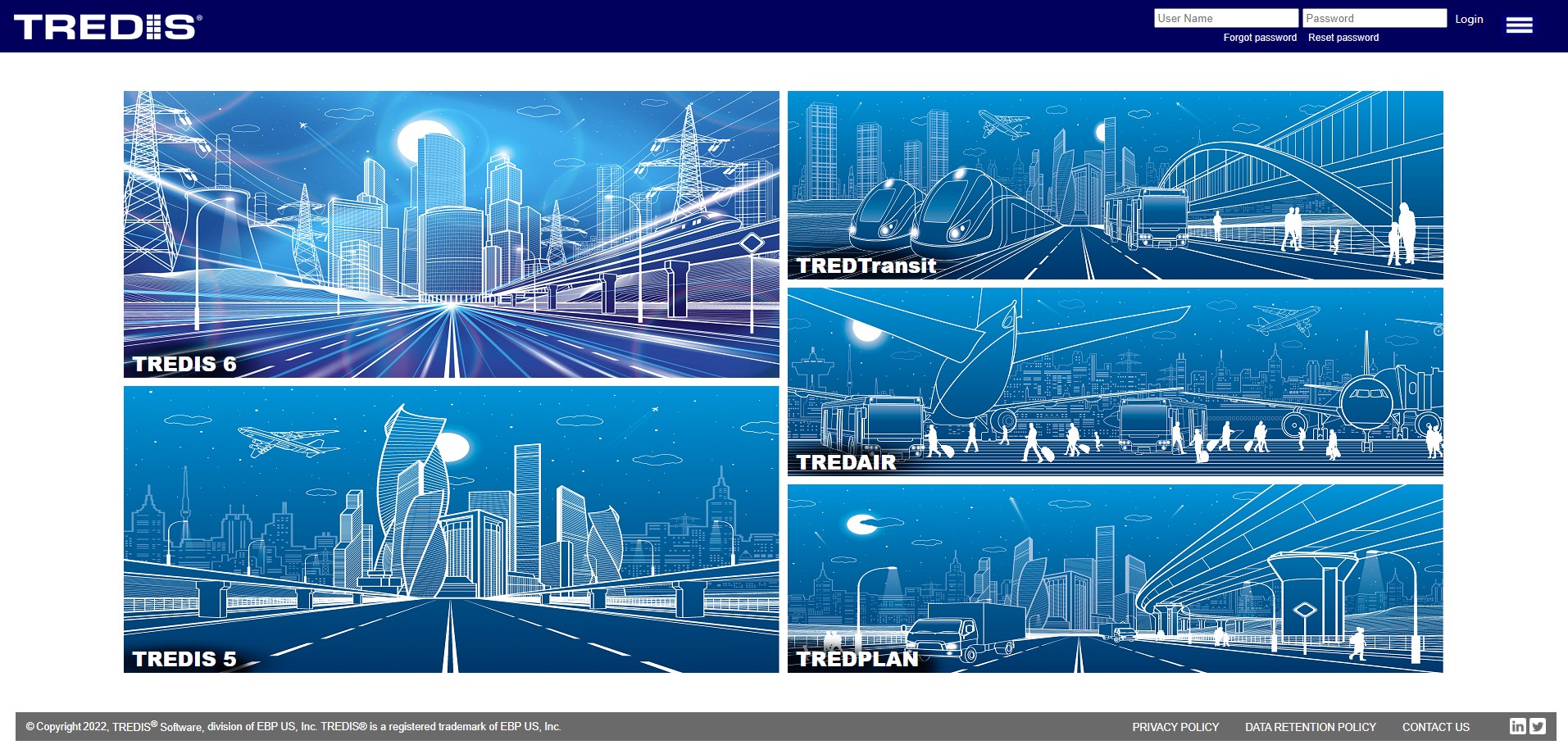
Using your web browser, access TREDIS by typing https://login.tredis.net and provide your user name and password in the
appropriate spaces on the Login Screen, as illustrated in the following figure.
Note that the first time you login to the TREDIS software, you will be prompted to accept the terms of use
and to change your password.
The icon
 with three (3) horizontal bars
at the top right of the screen opens a menu of information sources for TREDIS. From here you may access TREDIS
webinars, Tech Advisories, User Documents, View TREDIS News, FAQ's and the TREDIS Knowledge Base.
with three (3) horizontal bars
at the top right of the screen opens a menu of information sources for TREDIS. From here you may access TREDIS
webinars, Tech Advisories, User Documents, View TREDIS News, FAQ's and the TREDIS Knowledge Base.
Once you are logged in, the products for which you have subscribed will be shown in color, while those that are not subscribed will be in black and white monochrome.
TREDIS Steps
Every TREDIS Project follows the steps as shown in the navigation
bar in the next figure.

The following provides an overview of each step in the project analysis process:
- Project - Choose a project, start a new one, set project-level preferences, or manage projects.
- Timing - Set the construction and operations periods for the project and distinguish separate segments of travelers.
- Regions - Define regions using a map to create the economic model.
- Modes - Choose modes and purposes.
- Costs - Enter capital, maintenance and other building costs by facility.
- Travel - Input primary travel characteristics (trips, VMT, and VHT) and adjust rates and flows as needed.
- Access - Provide market access changes (if desired for your analysis) or add ad-hoc economic changes expected.
- Results - On first view, select analysis parameters and start run. Once run, see all reports and model outputs.
Note: Do not user the "back" button on our browser as this may
prevent proper data loading.
The three bar icon
at the upper right is the
Navigation Menu. The following are available from this menu:
| User Documentation | Technical and user documentation site that includes a link to this document. |
| Preferences | Opens the Preferences window. |
| Help | Opens a section of the User Manual relevant to the screen you are currently on. |
| User Manual | Opens a new browser window with the full User Manual. |
| Sample Import Spreadsheet | Downloads the current version of the Import Spreadsheet. |
| Product Menu | Directs you to the Product Menu screen, with tiles highlighted depending on your user licenses. |
| TREDIS 5 | Takes you to TREDIS 5 log-in. |
| Log Out | Logs out and returns you to sign-in screen. |
| TREDIS 6.0 User Manual | Return to Contents |
Preferences Window
The preferences window sets user preferences that apply to the Travel page and the Results reports. To change preferences, choose selections and click Save.
Preferences Window

Travel Characteristics: Input Preference
- Travel Speed means that on the Travel page you may enter speeds instead of entering both travel time and travel distance.
- Travel Time means that you must enter travel time and travel distance.
Travel Characteristics: Reliability Cost Estimation Method
This selector includes both a radio button and a dropdown menu. The radio buttons select whether you will provide only fraction congested, only buffer time, or Both on the Travel page, under the Congestion tab. The dropdown selects what format you will enter for buffer time if you are going to enter it. (If you select Fraction Congested, the dropdown has no effect.)
- Fraction Congested means that on the Travel page, under the Congestion tab, you only enter the fraction congested for modes where congestion is relevant.
- Buffer Time means that on the Travel page, under Congestion tab, you may only enter the buffer time associated with each trip (in fractions of an hour). Choose this by clicking the radio button next to the Reliability Metric Preference dropdown. On the dropdown, choose the way that buffer time is entered.
- Both means that on the Travel page, you enter both fraction congested and buffer time using the metric selected by the Reliability Metric Preference dropdown.
Travel Characteristics: Crash Entry Method
- Crash-Involved Vehicles means that on the Travel page, you may only enter rates and counts related to Crash-Involved Vehicles, not Crashes.
- Crashes means that on the Travel page, you may only enter rates and counts related to Crashes, not Crash-Involved Vehicles.
Results Page Defaults
- Impact Type dropdown selection defines the default Impact Type filter for Economic Impact reports. This is a default but can be changed on individual reports.
- Industry Aggregation dropdown selection defines the default level of aggregation of industries for Tracing/Validation and Economic Impact reports. This is a default but can be changed on individual reports.
- Discount Rates selections define the two discount rates that are immediately available for Benefit-Cost reports. If these are changed and saved here, the Benefit-Cost reports will reload with the new discount rates available.
| TREDIS 6.0 User Manual | Return to Contents |
Project Management
The Project is the basic unit of a TREDIS analysis and the start of the analysis process.

This status is helpful when submitting a project for a grant application so you know when the analysis was run and if it was last run prior to the submittal due date.
Next on the Project Page are four buttons:
For more advanced users, TREDIS provides you with the ability to manage the Projects in your Groups and to perform a bulk Import of Projects or a bulk Export of results.
Selecting and Defining the Project
Current Contract
The highest level of Project organization is by Subscription Contract. Contracts are used to associate projects to the
version of TREDIS Economic Data being used and to specify the associated geographies contained in
your subscription.
Current Group
Projects are next organized by Groups. To find an existing project, first select the desired Group from the pull-down
menu. If your organization has many groups, you can change the sorting order to be by Name (Group Name) or User.
Current Project
Once you have selected the appropriate Group, you can then find your Project in the pull-down menu. Again as
for the Group selection, you may change the sorting order to ProjectID, Name (Project Name), Project Owner, Sharing
Mode (private or shared (read only) with users within your account), Creation Date, or Last Modified Date.
Travel Analysis Type
Beginning with TREDIS 6, users now have the option to enter their project travel information using the Facility Based
method (legacy from prior versions of TREDIS) or to use an O-D Based method (origin-destination). The travel
analysis type is defined when creating the project and the selected type is shown here.
Alternatives
TREDIS automatically provides a Base Alternative and a Project Alternative when you create a project. You may change
the name by clicking the rename link. Enter the desired name and then click the update link or cancel to keep the current name.
Project Notes
This field allows you to record descriptive information about the current
project. To add or edit text in this field, click on the Properties button.
Created On
This field shows the date and time your project was created.
Analysis Complete
TREDIS informs you on the analysis status for the project. If the results are valid from previously running the Analysis, then
this field will show the date the analysis was last run successfully. If the analysis was never run or the last run was not successful
this field will show NA representing the results are not available without running the analysis again.
This status is helpful when submitting a project for a grant application so you know when the analysis was run and if it was last run prior to the submittal due date.
Next on the Project Page are four buttons:
|
Use the Create button to start a new project. This will open a popup window that lets you enter the name of your
new project and to select the Travel Analysis Type (Facility Based or O-D Based. The newly created Project
will be assigned to the Current Group.
 Facility Based
The Facility Based Travel Analysis Type is the traditional method for entering travel inputs used in prior
versions of TREDIS. This type provides the user with the most flexibility to control the
analysis process without limiting the input data screens or restricting access
to table fields.
O-D Based
The O-D Based Travel Analysis Type uses the concept of origin and destinations to specify the flow of travel
between regions including a standard, External, that is not specifically defined as a region. This travel type
eliminates the fraction of trips that are internal, incoming, outgoing, and through and replaces them with the more
specific ones showing the To/From regions. For a single region model (named Default Region), the fraction of
trips would be specified as:
|
|
|
To change the Project Properties, use the Properties button.
This popup window lets you add an optional Project ID, change the name of your Project, reassign its Group, or to add Project Notes. It
is here that you may change the sharing mode - toggle between private where only the project owner may see the project or shared, where
anyone with a user login within your account may see the project (read only). Shared projects may be copied.  If you want to share this project with a US DOT Grant Reviewer as part of a grant application, check the US DOT Review Enabled checkbox. This will
a grant reviewer to see a read only copy of your project. They may also make a copy which will allow the review to make adjustments to the mode factors
and travel inputs as part of their review. Any copies made by the reviewer will be visible to you as a shared project in the same contract and project group
as the original submitted project. The grant reviewer's name will appear with the new copied project.
Note: To remove permission for a grant reviewer to see your project uncheck the box and press the Save button. |
|
|
Use the Copy button to make a copy of the Current Project. In the
window that opens, enter the name for the copied Project.
|
|
|
The Delete button lets you delete the current Project. You will be given
an opportunity to confirm the deletion. Press OK to delete the Project or CANCEL to keep the Project. Only the project owner
may delete their project(s).
Warning: Once a project is deleted, it cannot be recovered. |
For more advanced users, TREDIS provides you with the ability to manage the Projects in your Groups and to perform a bulk Import of Projects or a bulk Export of results.
|
The Group Options function allows you to organize, rename, delete, create backups and export results for
multiple projects. Click the Group Options button at the left for more information
|
|
|
The Import Projects button takes you to a screen where you may upload multiple projects at once using a spreadsheet.
The "TREDIS Project Import Template" spreadsheet is available by clicking on the on the menu icon at the top right of the screen and select the Sample Import Spreadsheet or click on the Import Projects button and select the Import Project Template Spreadsheet link. Click on the Import Projects button to the left on this page for more information on using this feature. |
|
|
The Compare Projects button opens a new window that lets you see the results from multiple projects in the current contract and current
group. For more information click on the image of the button at the left
|
|
|
The Multi-criteria Compare button opens a new window that lets prioritize projects with a specialized tool that can weight factors such as VMT savings,
economic impacts, and equity considerations. For more information click on the image of the button at the left
|
| TREDIS 6.0 User Manual | Return to Contents |
Project Management – Group Options
In TREDIS, each analysis of a Base-Project alternative pair is called a Project, and projects are organized into Groups. The Group Options window allows you to manage the organization of their projects. TREDIS also allows performing multi-project tasks, such as exporting results, changing sharing levels, and deleting multiple projects.
Group Options Window

Modify Group
The controls in Modify Group section let you change the Groups (not the projects themselves) for the current contract you are working in.
Use the dropdown menu to select a Group to modify.
- Create New Group. Create a new Group. This will open a popup window that lets you enter the name of your new Group.
- Rename. Rename the current Group selected. Then press the Rename button, which will open a window to enter the new name.
- Delete. To delete a group, select the Group to delete from the dropdown menu, then press the Delete button. A window will open to confirm that you want to delete permanently.
Selecting Projects
In the Group Options window, before you can perform any bulk operations on projects listed in the Modify Selected Group section or any of the buttons to the right, you must select any number of projects in the current Group at the same time to perform those actions on.
Group Options Window with Projects Selected

Before you select projects, make sure the current Group you want to operate on is active. This can be done by choosing a Group from the Modify Selected Projects section, with the Filter by Group control. Doing this will change the Projects listed in the pane at the bottom. Alternatively, you can select all projects associated with the current contract by selecting All Groups.
The available projects to select or deselect are listed at the bottom of the window along with their details. You can select them using any combination of these methods.
- Manual selection. You can always click the checkbox to the left of each project name to select or deselect it.
- Toggle all. Check the box at the top of the pane to select (or deselect) all of the projects listed.
- Range Selection. In the Range Selection section at the top right of the window, enter the first and last row numbers for the projects you wish to select, and the system will automatically select these projects.
Modify Selected Projects
You can perform operations on all of them using the options in the Modify Selected Projects section of this window.
Use the Filter by Group dropdown to select the desired Group. You also have the option to select all groups by selecting All Groups from this menu. You will notice that the list of projects below will change based on the filter settings.
After selecting projects to operate on using the options described in the section above, you can perform the following actions on all of them:
- Assign to Different Group. Use the dropdown menu Assign to a Different Group to select a Group to reassign the select projects, and click the Assign button. If you have filtered your projects by a specific group, they will disappear from the current view to reflect the change.
- Change Sharing Mode. Use the dropdown menu Change Sharing Mode to change projects from Private to Shared (or Shared to Private), and click the Change button.
- Delete Selected Projects. Delete any projects currently selected. You will be asked to confirm before this is executed. This process may take some time, and a progress message will appear to the left of a button labeled Cancel Deletion.
Bulk Operation Buttons
Other important operations that result in an exported Excel sheet can be accessed via the buttons to the right of the Modify Selected Projects section. Each of these buttons launches its own window to launch the operation.
Click on the names of the buttons below for detailed instructions on the operation.
 |
Run the selected projects and export a summary Excel spreadsheet to be sent to e-mail.
|
 |
Create a back-up Excel spreadsheet of selected projects for re-import later.
|
 |
Produce an Excel spreadsheet combining multiple Results reports for the selected projects.
|
| TREDIS 6.0 User Manual | Return to Contents |
Project Management - Import Projects
The project import functionality in TREDIS is a powerful feature that can be used to recreate project backups and, for advanced users, to create projects in bulk. In either case, TREDIS projects are read in from an Excel file in the Import Spreadsheet format.
The Import Spreadsheet
The Import Spreadsheet in TREDIS is an Excel file with a defined structure. You can see a sample by clicking on the on the menu icon at the top right of the TREDIS screen and selecting Sample Import Spreadsheet.
The spreadsheet has its own documentation on the Read Me and Tabs and Columns tabs. (Black tabs are documention, green tabs are necessary, and gray tabs are optional.)

Troubleshooting Import
If you've never imported a project before, we recommend that you back up a project first. Once the back-up is downloaded, open the Excel file and read the documentation (on the black tabs at the far left). You should also take a minute to browse the green and gray data tabs to see how data is organized and presented. This will help you avoid errors in import and understand the purpose of individual tabs. Common problem areas are discussed below.
Preferences
On the User Preferences tab, the Preference Settings values should match your current user Preferences. To change your current User Preferences, click on the on the Navigation Menu (at the top right of the TREDIS screen) and select Preferences.
Dollar Year
On the Project tab, the Constant Dollar Year should be the same for all projects and match the year of the Contract you are trying to import to.
Unique Project Names in a Group
The names of any projects being imported cannot be the same as any projects in the group being imported into. You can always add a suffix with the date if you are unsure if the projects you're importing will have a unique name. (For example, "My Project" could become "My Project 2024-12-13".) If you need to update project names in Excel, you will probably want to use the Find-Replace functionality, with the Within: Workbook option selected, as in the screenshot:

Missing Data on Green Tabs
Make sure data is entered for all green tabs in the Import Spreadsheet (or for the OD version of the tab, if appropriate). An exception is the Costs tab. TREDIS cannot provide default Costs data, but the tab can be left blank if you do not intend to analyze cost data. (This might limit your analysis. For example, you won't be able able to calculate a benefit-cost ratio without costs input.)
Import Steps
This section steps through the screens and operations to import projects in the TREDIS application.
From the Project page, start the process by clicking the Import Projects button at the bottom of the screen.


In the Upload New Projects window, you will be presented with a list of all projects that are contained in the spreadsheet. On this screen, check off projects you want to import. Then click the Import Selected Projects button.

The Import Options window will appear. First, select which Project Group to import the projects. You can create a new group on the fly by entering a new group name and clicking the Create button.
Another radio button toggle allows you to decide if empty values will be filled by a default or stop the import process.
Once the project group is set and any desired settings adjusted, press the Start Import button to initiate the process.

As the projects are imported, their status you will see the status on the project list screen.
| TREDIS 6.0 User Manual | Return to Contents |
Project Management - Compare Projects
The Project Comparison feature allows you to compare analysis results across up to 30 selected projects. It can be used as a sanity
check on the validity of your inputs to TREDIS and to easily find significant differences with respect to economic impact and benefit costs.
Project comparison is included in standard TREDIS subscriptions, but not available in the TREDIS MBCA, Trial, or University accounts.
The left side of the screen is a menu that allows you to move between comparison reports.
If you do not see a project in the list, go back to the project screen and check to see if the project has been analyzed. You may either click on results to run the analysis, or if you have multiple projects to analyze, use the multi-run feature within group options on the project page.
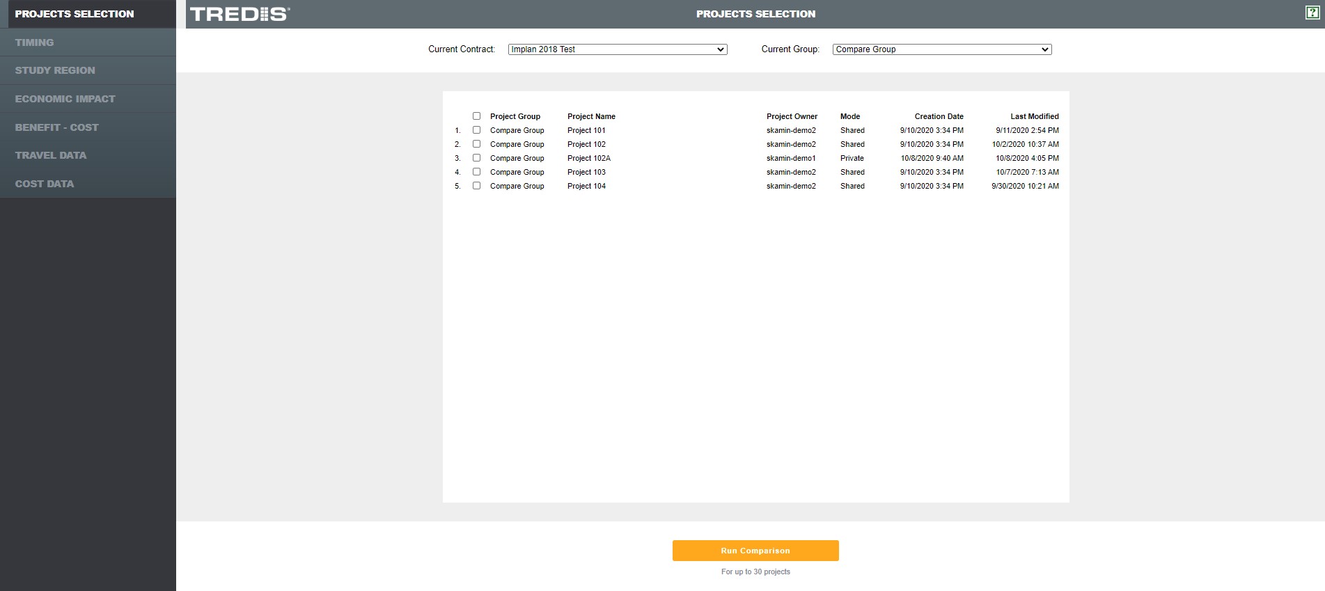 Select the projects you wish to view, up to a maximum of 30, and then click on the Run Comparison button. You will then be directed to the
Economic Impact Comparison Screen.
Select the projects you wish to view, up to a maximum of 30, and then click on the Run Comparison button. You will then be directed to the
Economic Impact Comparison Screen.
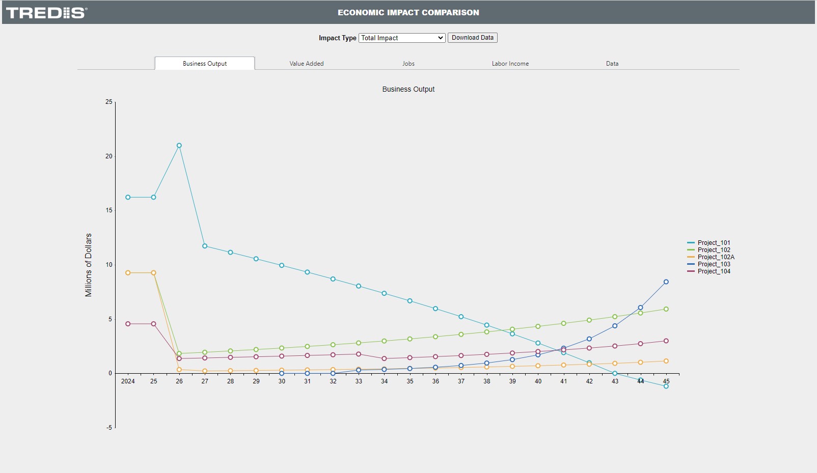 As seen on the picture above, you may select the Impact Type from the drop down menu, to show the total impact, or filter by construction,
operations, market access, or contingent development. Clicking on the Download Data button will export the data used in creating the graphics
on the page for the impact type selected.
As seen on the picture above, you may select the Impact Type from the drop down menu, to show the total impact, or filter by construction,
operations, market access, or contingent development. Clicking on the Download Data button will export the data used in creating the graphics
on the page for the impact type selected.
The chart on the screen will present business output ($M), value added ($M), Jobs, and Labor Income ($M) over time, depending on which tab is selected. The data tab shows a simple table of the results for the results year selected in the analysis settings.
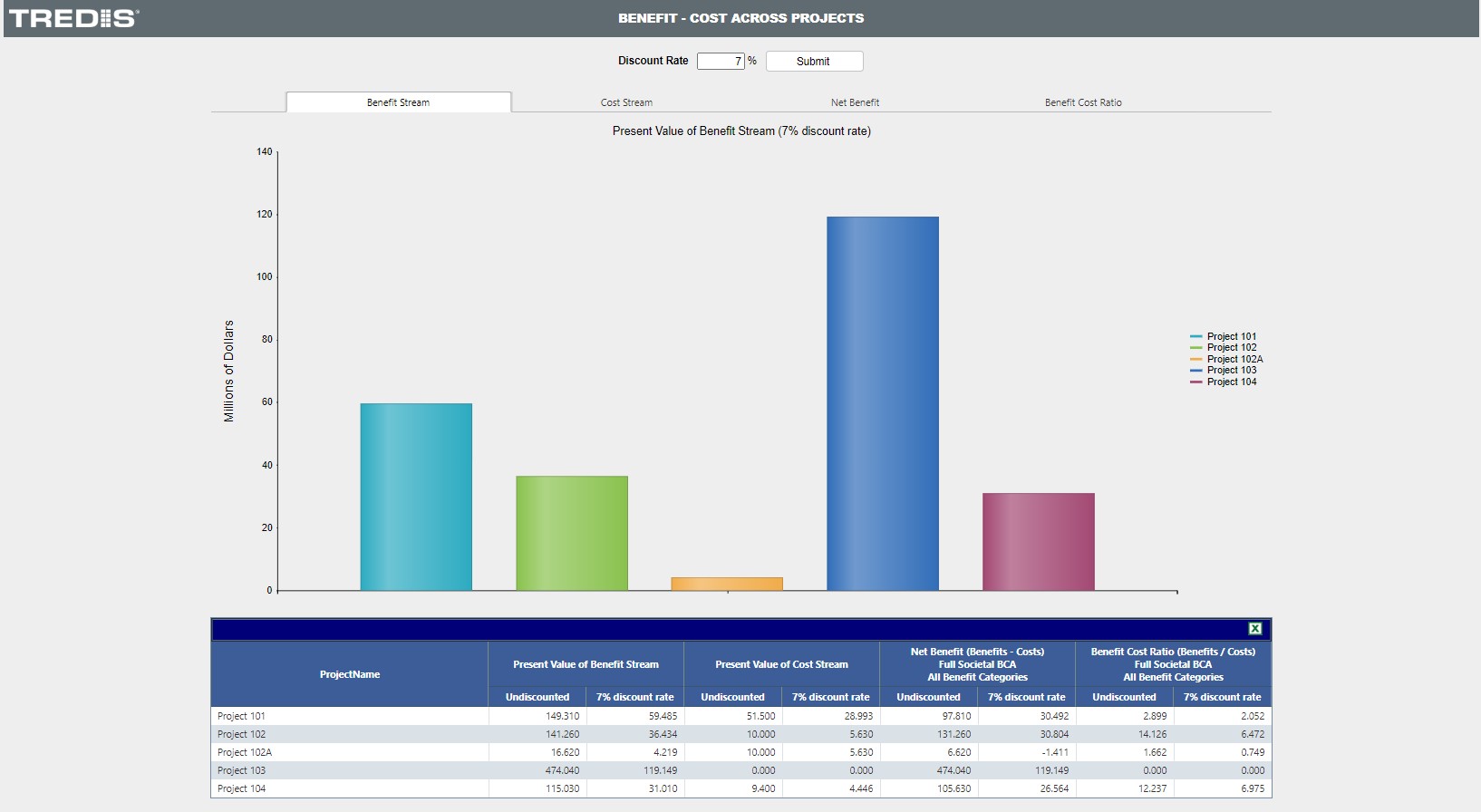 Clicking on the Benefit-Cost tab on the left menu, presents the graphical view of the Benefit Stream, Cost Stream, Net Benefit, and
Benefit Cost Ratios, with a table of the data at the bottom of the screen.
Clicking on the Benefit-Cost tab on the left menu, presents the graphical view of the Benefit Stream, Cost Stream, Net Benefit, and
Benefit Cost Ratios, with a table of the data at the bottom of the screen.
At the top of the screen, you may change the discount rate by entering a value and clicking the submit button. Entering 0 will show the undiscounted values.
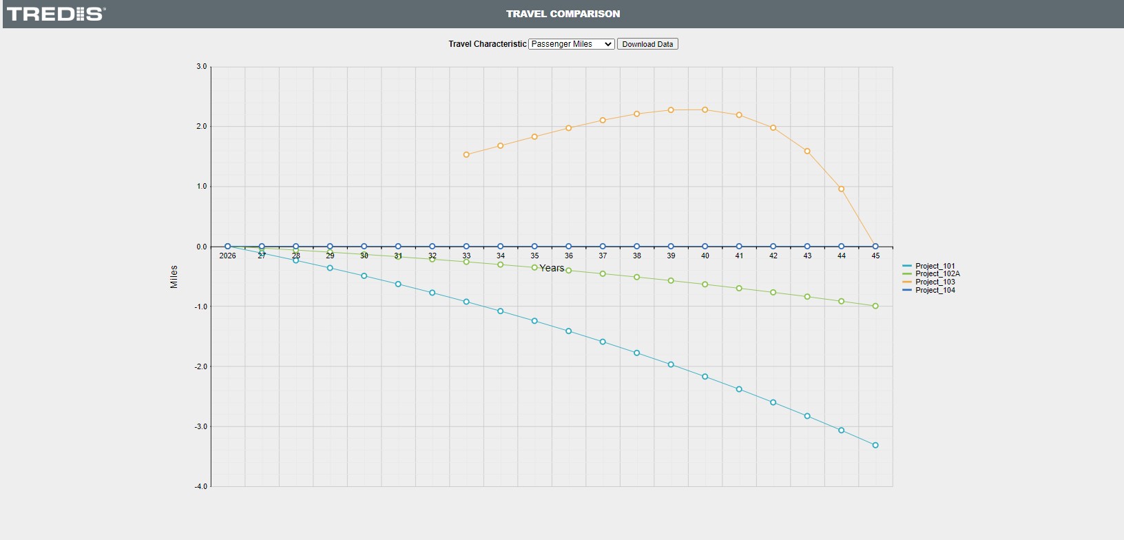 The Travel Comparison screen shows the travel inputs (difference of project less base) over time for
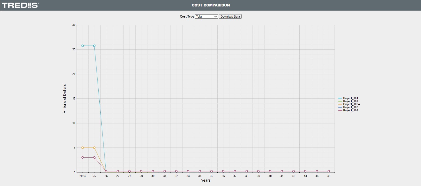 The Cost Comparison screen shows the total costs, construction costs, or operational costs over time for the selected projects.
Use the dropdown menu to select which cost type is of interest and the Download Data button for the raw data.
The Cost Comparison screen shows the total costs, construction costs, or operational costs over time for the selected projects.
Use the dropdown menu to select which cost type is of interest and the Download Data button for the raw data.
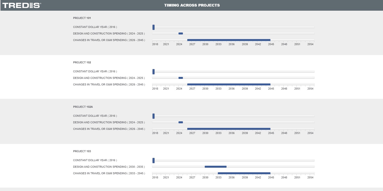 The Timing screen shows the construction and operations periods of each selected project, along with the constant dollar year used to enter data.
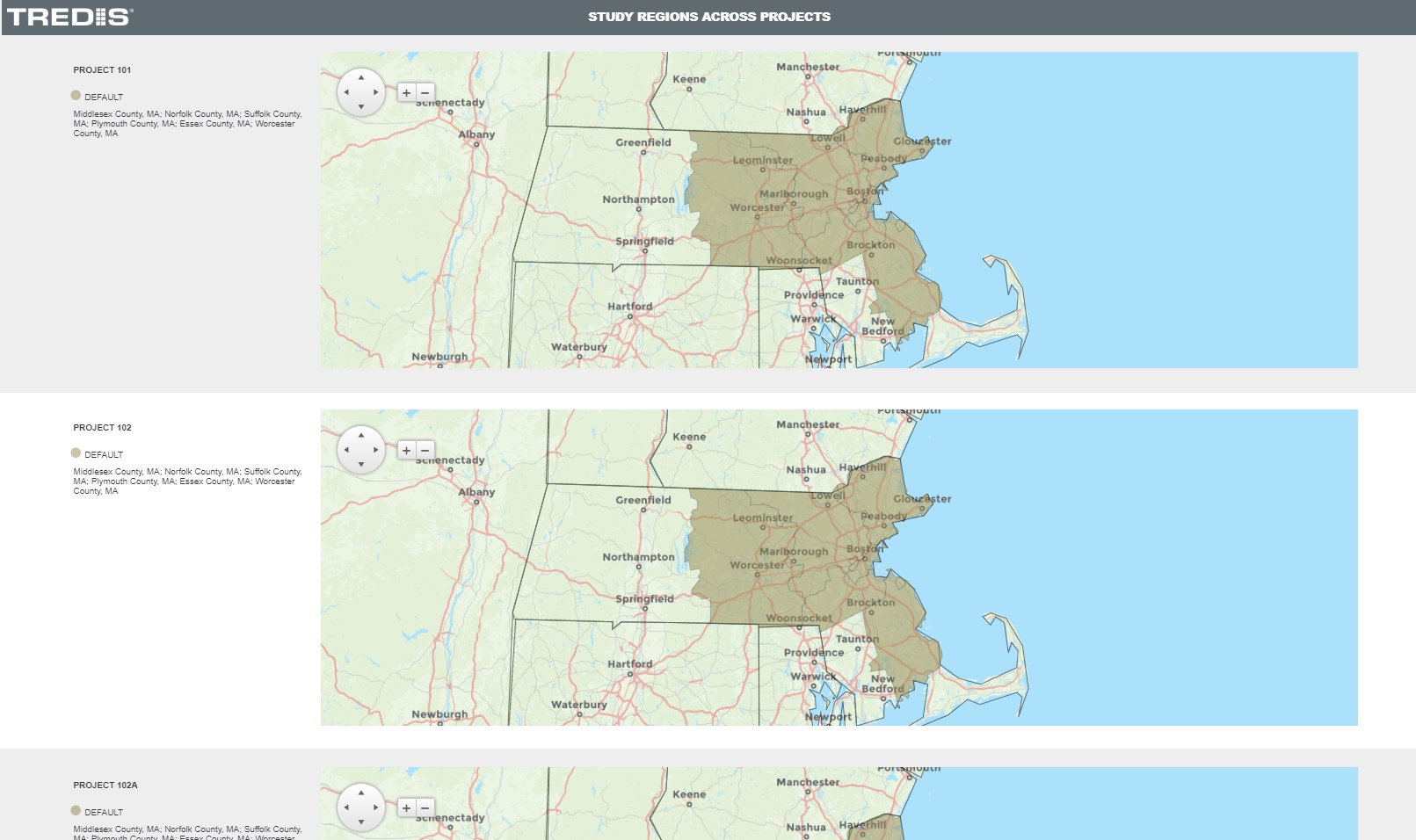 The Study Region tab present a list and a map of the study regions for each selected project.
Project comparison is included in standard TREDIS subscriptions, but not available in the TREDIS MBCA, Trial, or University accounts.
The left side of the screen is a menu that allows you to move between comparison reports.
Project Compare - Project Selection
When you first click on the Compare Projects button, a new window opens which lists all projects that have been analyzed for the current contract and project group. At the top of the screen, you are able to select another contract or group if they exist, which will repopulate the project list.If you do not see a project in the list, go back to the project screen and check to see if the project has been analyzed. You may either click on results to run the analysis, or if you have multiple projects to analyze, use the multi-run feature within group options on the project page.
Project Compare - Economic Impact Comparison
The chart on the screen will present business output ($M), value added ($M), Jobs, and Labor Income ($M) over time, depending on which tab is selected. The data tab shows a simple table of the results for the results year selected in the analysis settings.
Project Compare - Benefit Costs Across Projects
At the top of the screen, you may change the discount rate by entering a value and clicking the submit button. Entering 0 will show the undiscounted values.
Project Compare - Travel Comparison
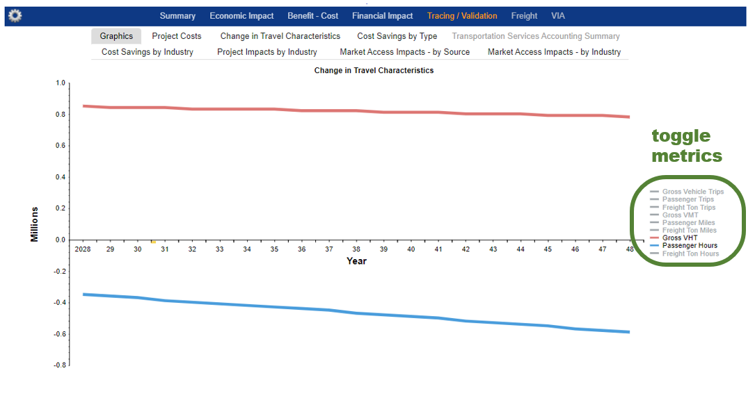
- Gross Vehicle Trips
- Passenger Trips
- Freight Ton Trips
- Gross VMT
- Passenger Miles
- Freight Ton Miles
- Gross VHT
- Passenger Hours
- Freight Ton Hours
Project Compare - Cost Comparison
Project Compare - Timing Across Projects
Project Compare - Study Regions Across Projects
| TREDIS 6.0 User Manual | Return to Contents |
Project Management - Multi-Criteria Compare
The Multi-Criteria Compare feature allows you to prioritize projects by weighting competing priorities.
The left side of the screen is a menu that allows you to move between comparison reports.
The Projects tab on the Projects Selection page is the landing screen.

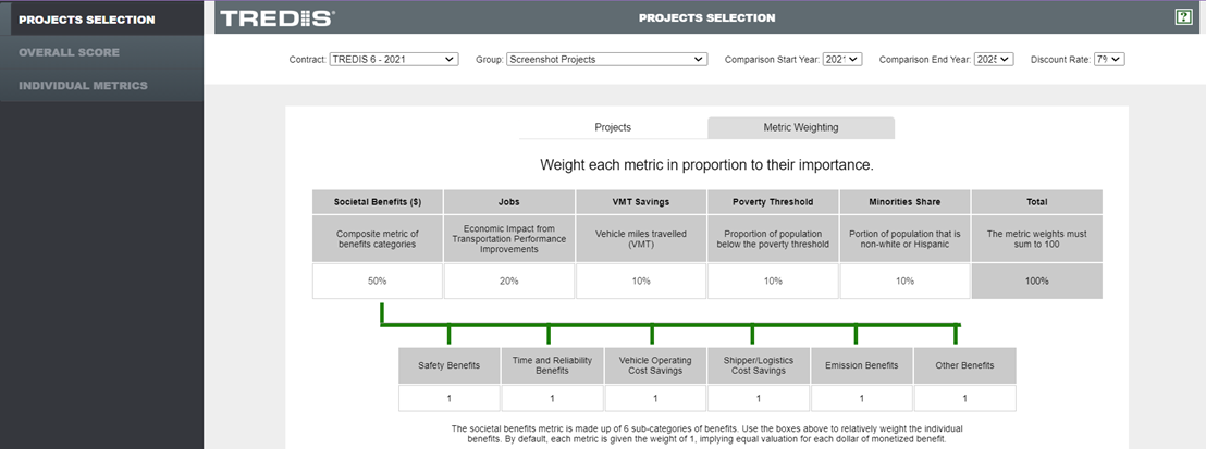
On the Metric Weighting tab, select the weights for each category of evaluation. The upper tier of weights entered must add to 100%. The bottom tier is only the relative weighting of factors within the larger Societal Benefits category. These are weighted just with integer weights, but there is no constraint on their sum.
The Overall Score screen has two tabs, the Table tab and the Chart tab. The Table tab displays the primary results of the analysis.

The Charts tab shows scoring data as a bar graph.
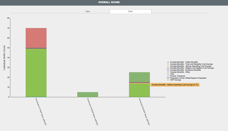 The legend at right allows the user to toggle on or off components of interest, and hovering over a bar section will display a score (as
in the illustration, where a label for the Vehicle Operating Cost Savings appears). For Societal Benefits, this score is further scaled
to represent its final contribution to the individual score.
The legend at right allows the user to toggle on or off components of interest, and hovering over a bar section will display a score (as
in the illustration, where a label for the Vehicle Operating Cost Savings appears). For Societal Benefits, this score is further scaled
to represent its final contribution to the individual score.




Once you have made your changes, click the Save Selected button to return to the Modes page.
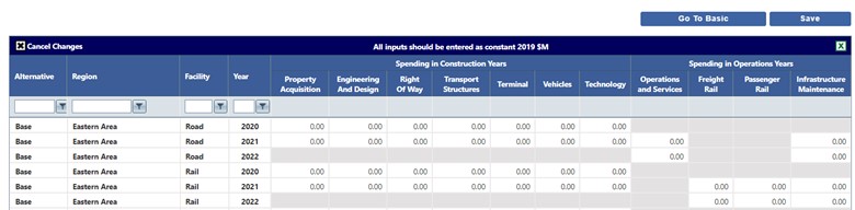
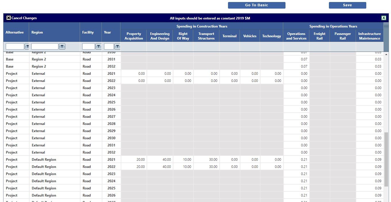
If there are many rows of inputs, you may want to filter by entering a filter argument in the fields below the column names, then clicking the filter button to choose a type of filter.
Notice that the Spending in Construction Years are available to input for every year of your Construction, and the Spending in Operations Years are available for input for every year of Operations, both set in the Timing screen.
Engineering and Design - Soft costs of construction, including planning, analysis, legal, architectural, engineering, and design work.
Right of Way - Earthmoving, grading, drainage, and paving. For railroads, this includes all expenditures on the laying of rails; for airports, this includes runway construction.
Transport Structures - Construction of culverts, road bridges, flyovers, railroad bridges, and marine docks
Terminal - Operations offices, maintenance facilities, airport/bus/rail terminals, and storage buildings
Vehicles - Acquisition of rail cars and engines, ferries, airplanes, barges, or maintenance or service vehicles
Technology - Intelligent transportation systems (ITS), communications equipment, electric vehicle infrastructure
Passenger Rail - Costs for operations for Passenger Rail, including systems operation, or incident management
Freight Rail - Costs for operations for Freight Rail, including systems operation, or incident management
Infrastructure and Rehabilitation - Crack repair, repaving, or vegetation control; also includes vehicle servicing.


"In-Model" trips represent trips that were undertaken in the Base alternative as well as the Project alternative, and which are assumed to have the same value for the people undertaking them.
"Induced" trips represent new trips undertaken in the Project alternative because travelers found new travel conditions that made a journey worthwhile when they were not in the Base alternative.
TREDIS assumes that the economic conditions are the same in any tested alternatives for a single scenario, so a different level of population and employment should not be the cause of trip "imbalance."
In some cases, a change in the number of trips between Base and Project alternatives is represented by in-model changes or a change in what inputs represent.
For example, if journeys made as one trip in the Base alternative are reported as two in the Project alternative – for instance, if a single bus trip now includes a transfer – the difference in the number of trips should be considered "in-model" because they don’t represent new journeys.
Another case where differences might be in-model are in mode switching. If some percentage of commuters that drive have switched to bus, the number of bus passenger trips is likely to have risen, but the difference is "in-model" since only the mode has changed.
Induced trips are journeys that were not available or feasible in the Base alternative. For example, if highway speeds have improved due to an additional lane in the Project alternative, more trips may be undertaken versus the number in the Base alternative because of the marginal cost in time.
Differences in trip counts due to technical constraints in a microsimulation model should be handled before TREDIS rather than by the Trip Balancing window.
The Travel screen in Figure 1 shows increases in total trips between the Base alternative and the Project alternative. The occupancy rates (on the following tab) for all modes and purposes have been set to 1.0 to simplify the example, so that vehicle trips are equal to person trips.
The Trip Balancing button is orange because it needs attention.
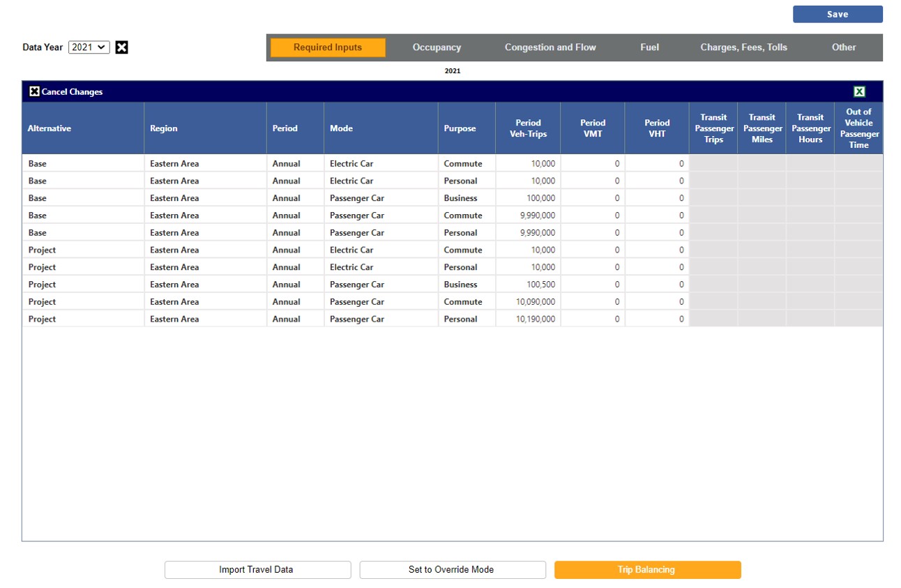
In Figure 1, the number of Business trips rises from the Base alternative to the Project alternative by a total of 500. Dividing by the number of Base alternative Business trips, TREDIS finds a 0.5 percent increase (500/10,000). Though there are two modes used for Commute – Electric Car and Passenger Car – they are considered together for purposes of Commute travel, which in total rises 1 percent (change in total commute trips divided by over total commute trips in Base alternative, or 100,000/10,000,000), while total Personal travel has risen by 2 percent.
In Figure 2, "50%" in the Overall % Induced column has been entered by the user to indicate that half of new traffic – any increase, regardless of purpose – is considered induced. This will be applied to each of the four modes shown in the other columns during Run Results.
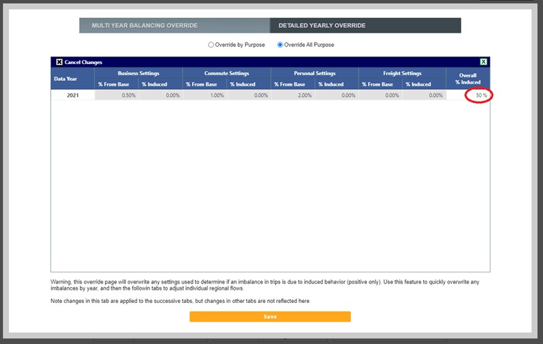
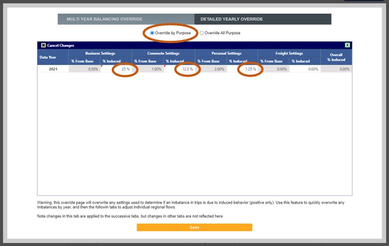
Figure 3 shows how, by toggling to Override by Purpose, the induced percentage can be set separately by year for each purpose (Business, Commute, Personal, and Freight), though in this case there is only 1 year.
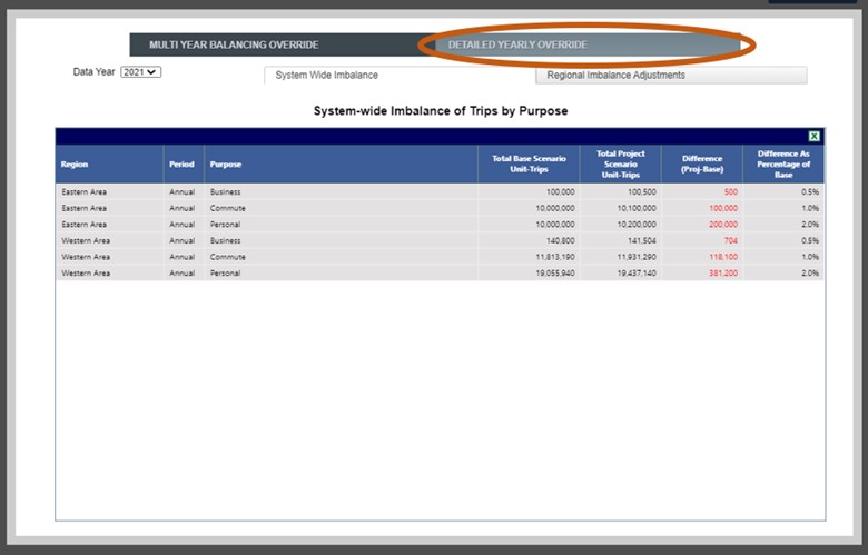
By selecting Detailed Yearly Override, you may reach the screen in Figure 4 showing the System Wide Imbalance tab, to see differences by region and period.
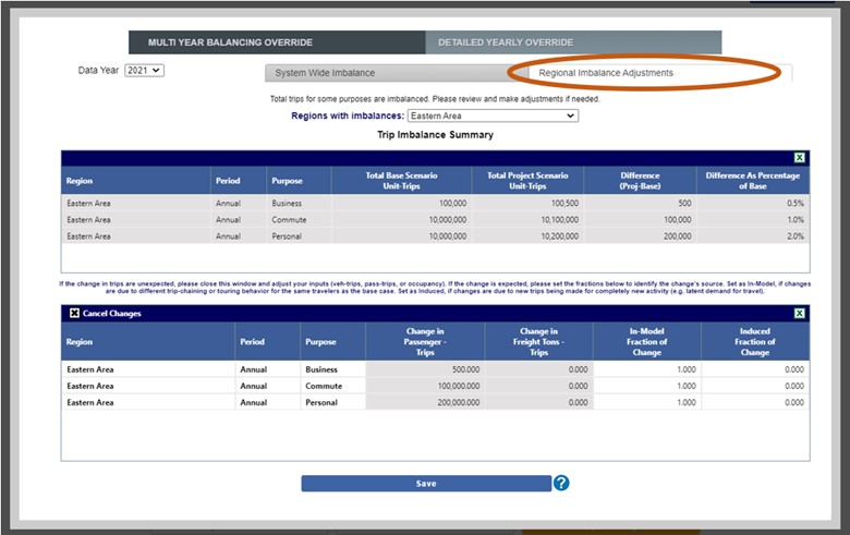
In Figure 5, the Regional Imbalance Adjustments subtab opens a table where the percentage of induced activity can be set by purpose, by year, by region and by period (the most granular input structure).


You will notice that the Run Analysis button has turned blue indicating that the analysis has completed and the Run Freight is yellow indicating this analysis still needs to be run.
Please review and change the following settings for running you freight analysis:
Once you have specified the settings for the freight analysis, press the Run Freight button. Once completed, you will again be left on the summary screen, but will now have access to your freight results.
View results or Run Freight analysis
You may now review the economic, benefit-cost, and financial impact results or you may go back to the
settings screen - click on the gear icon, to run the freight analysis.
Once you have specified the settings for the freight analysis, press the Run Freight button. Once completed, you will again be left on the summary screen, but will now have access to your freight results.

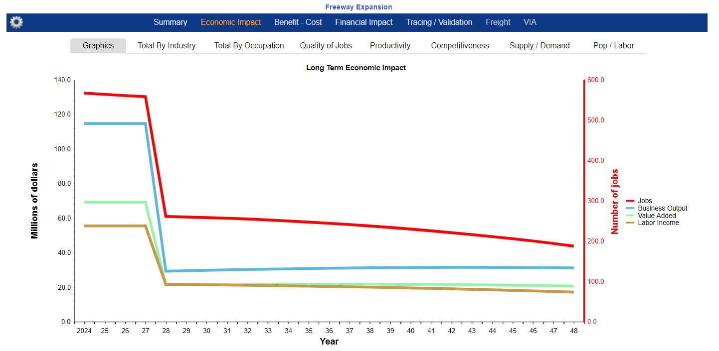
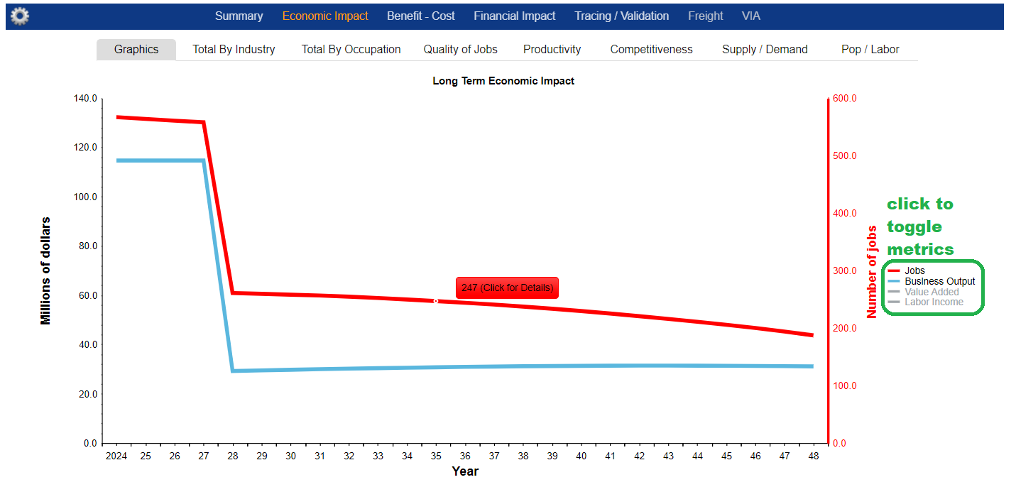
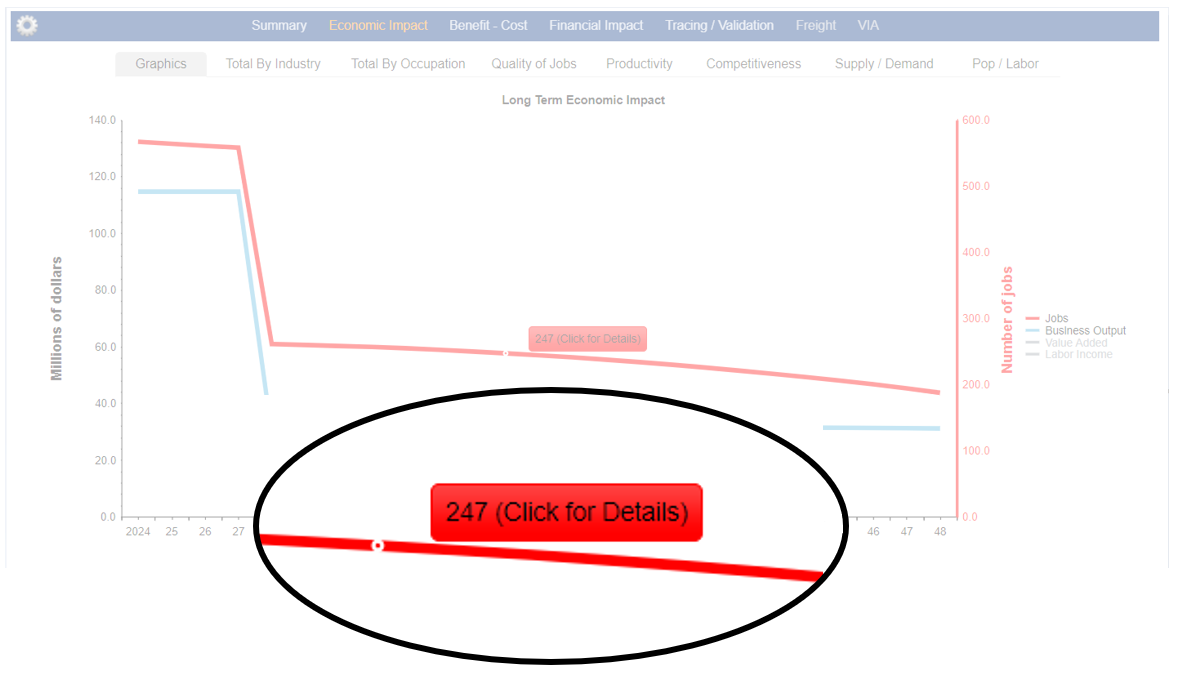
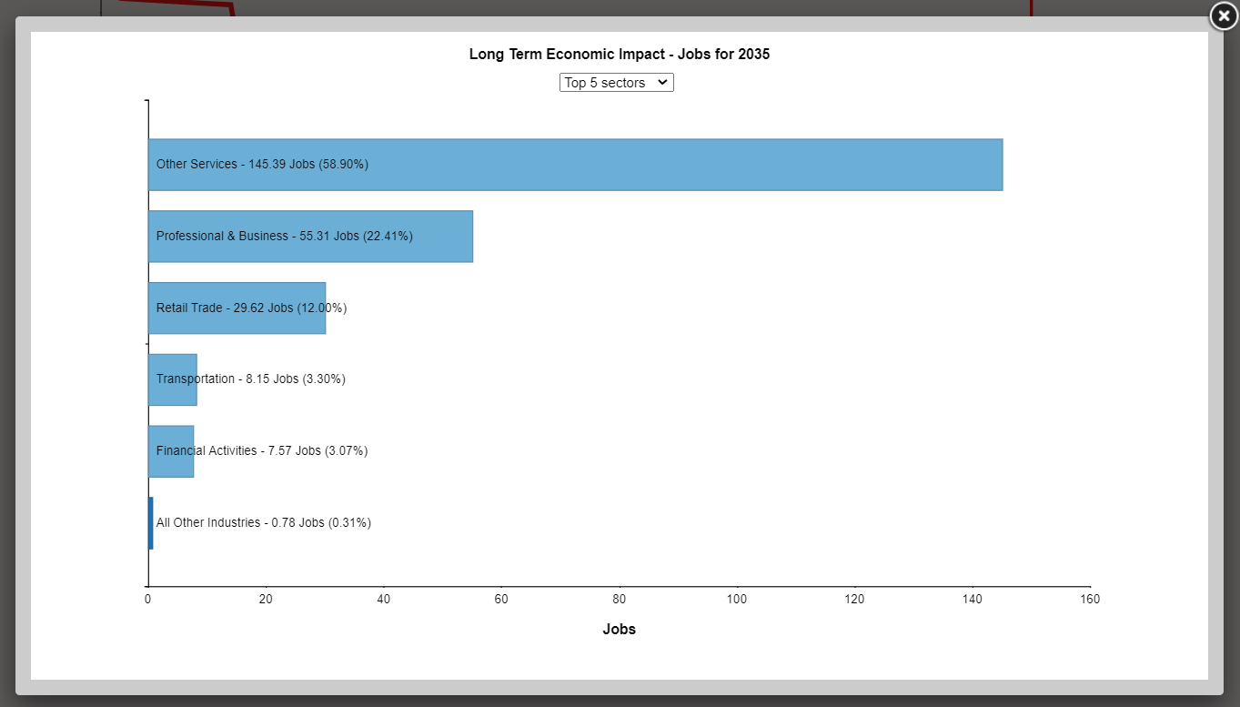
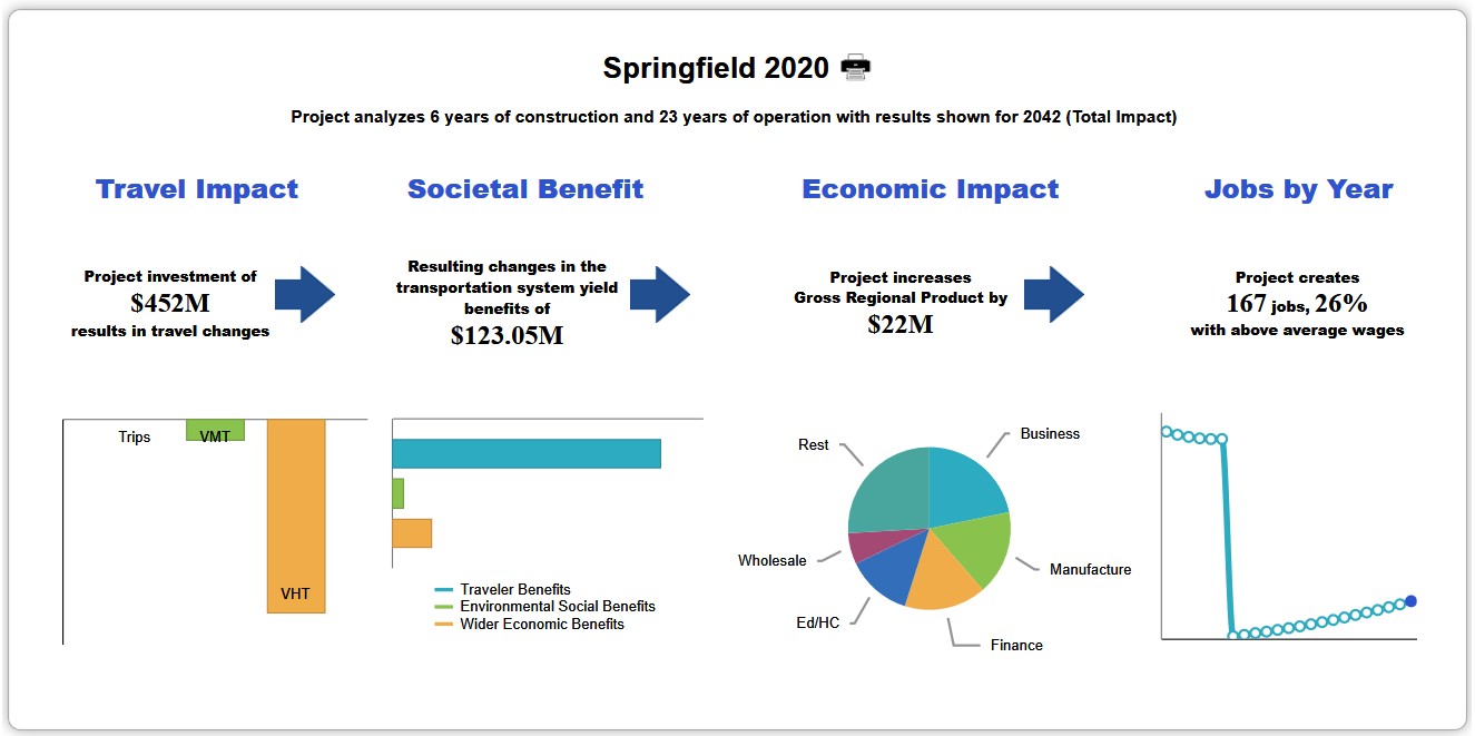
Total by Industry
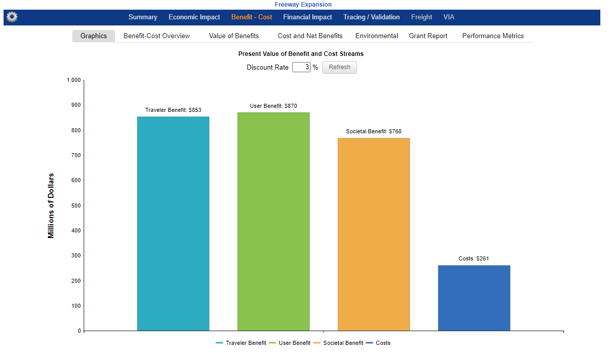
The Graphics and Benefit-Cost tabs present three different groupings of benefits with the Societal benefit encompassing total benefits. The following sections explain the benefit groupings and their components in detail.
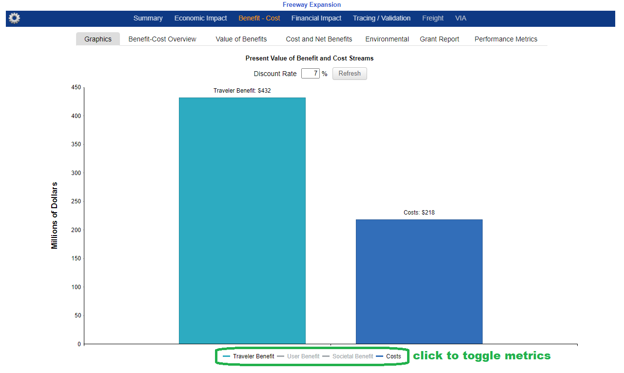
Interactive feature: Toggle on and off metrics by clicking on them in the legend. For example, User Benefit and Societal Benefit may be toggled off to see only Traveler Benefit and Costs.
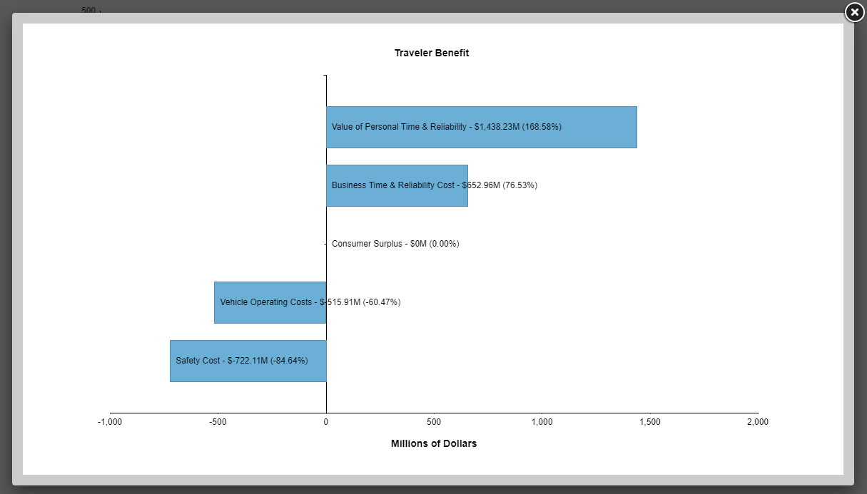
Interactive feature: Click on a Benefit bar reveal a disaggregation by category. Clicking on the Traveler Benefit bar above, for example, shows the breakdown between categories:
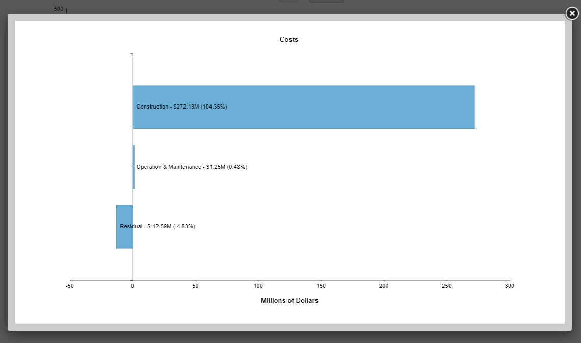
Interactive feature: Click on the Costs bar to reveal a disaggregation by Costs categories:
Interactive feature: Update the Discount Rate and click Refresh to change the discount rate for all measures.
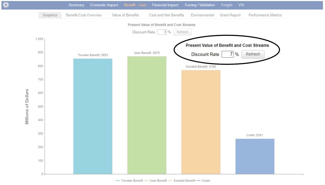
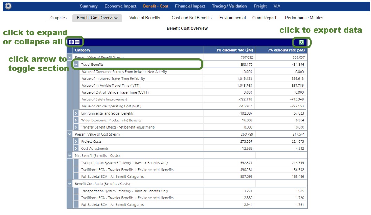
All values are in present values (discounted) terms, in millions of dollars.
See the Benefit-Cost FAQ for details on the signs of Benefit and Cost categories.
The left tab provides aggregations by year while the right tab provides aggregations by mode-purpose.
Interactive feature: Dynamically set the discount rate with the drop down.
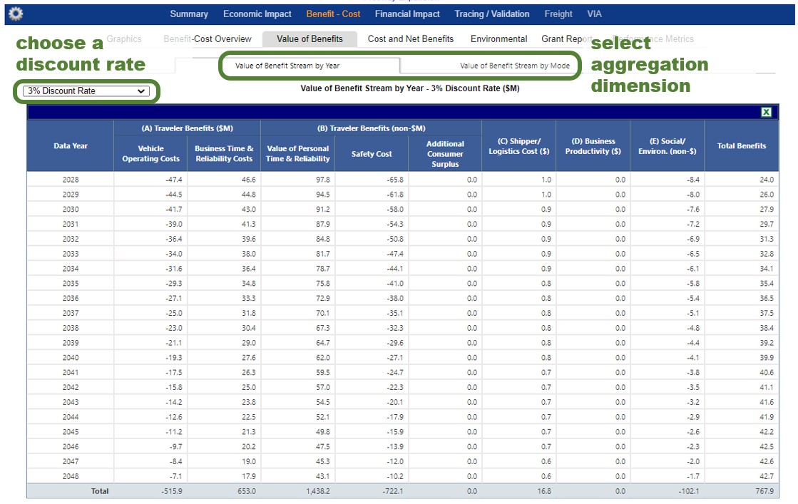
Monetized benefits include expenditures or savings on vehicle operating costs, and represent actual money transfers. Whereas externalities (safety and the environment) are monetized to capture the full range of benefits, even though these benefits only represent an approximate measure of value.
For example, vehicle operating costs include user expenditures on fuel, maintenance (tires, brakes, etc.), and vehicle depreciation per mile. On the other hand, reduced commute times benefit users, and are monetized to capture the total benefit to society of the project (relative to the cost), despite no monetary transfer to the commuter.
As elsewhere, keep in mind that Benefits refers both to positive benefits and negative (dis)benefits.
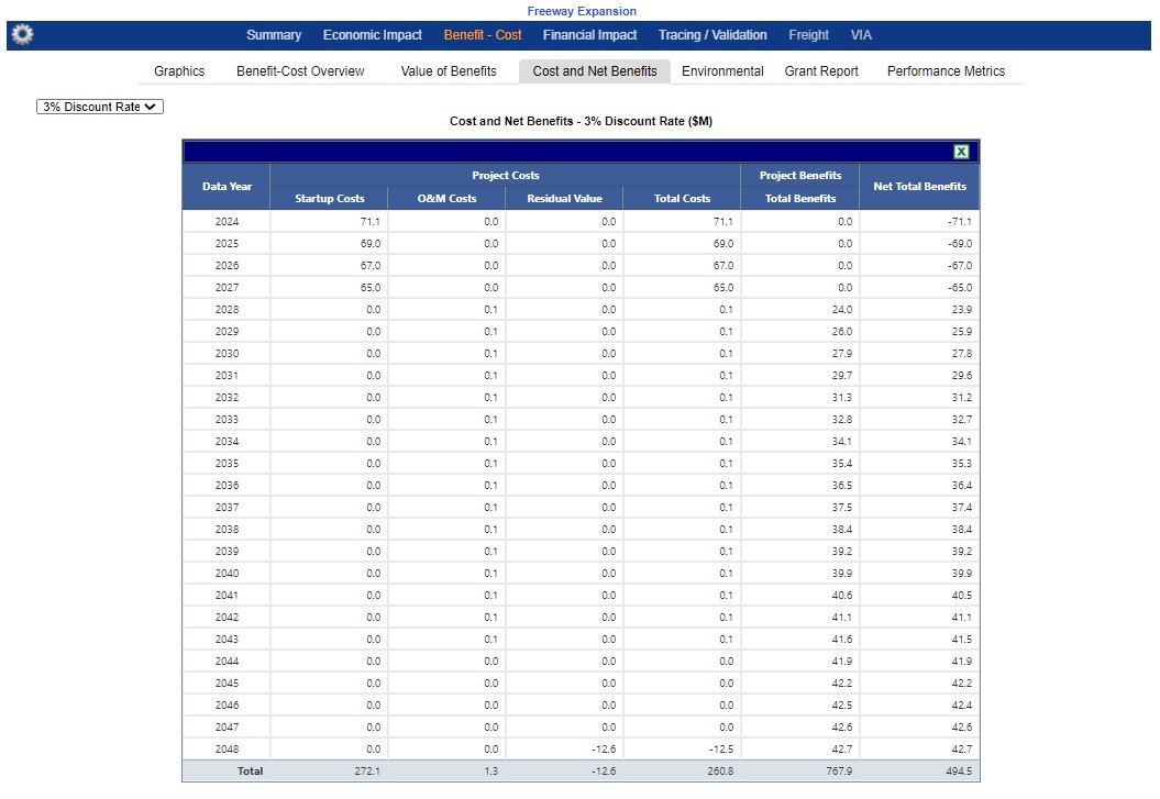
All figures are in millions of dollars. The categories are monetized unless noted otherwise.
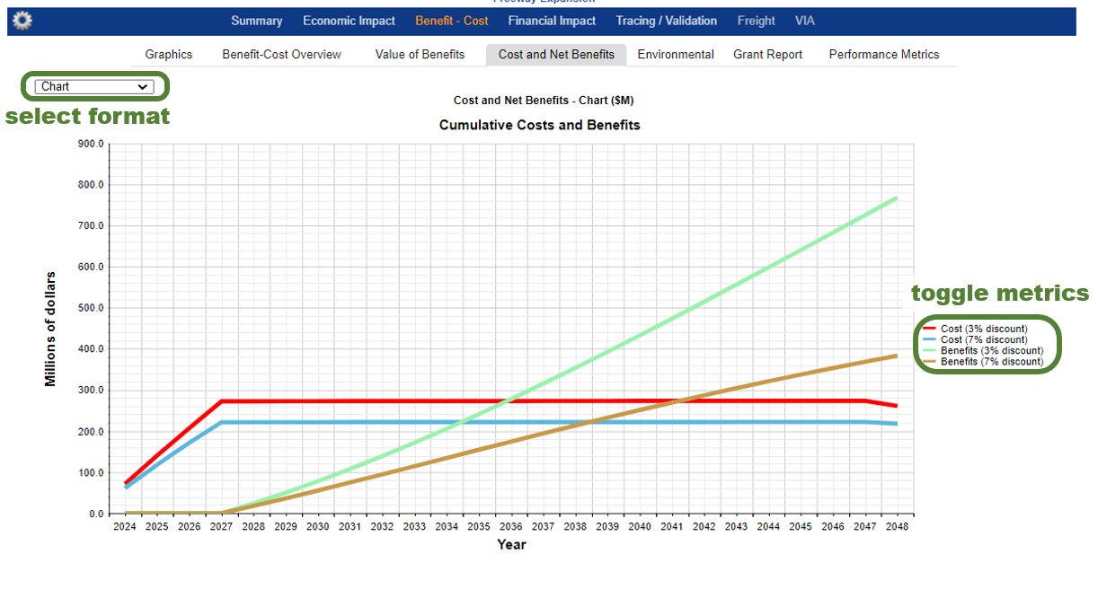
Interactive feature: Clicking on the metric descriptions in the legend toggles them on or off.
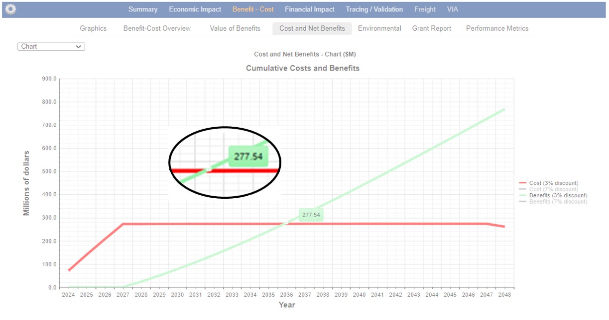
By toggling off the metrics showing Benefits at 7% and Costs at 7%, we can see just the rates for 3%. Then, hovering over the line for benefits, we can see individual year values.
This is often useful for quickly identifying the year that cumulative benefits overtake cumulative costs.
Tabs under the Environmental show emissions by year in metric tons, the value of emissions by year, and the value of emissions by mode-purpose.
For the value reports, the drop-down menu in the upper left allows you to choose a discount rate.
As with other benefits and savings in TREDIS, the environmental benefit may be negative to represent a disbenefit due to more pollutants.
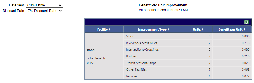
For these calculations, induced trips’ full cost is counted. (Compare with the calculations for Induced Benefit, where only half the benefit is assumed to be enjoyed by consumers, since that calculation is for the user benefit.)
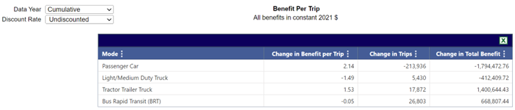
Dropdown menus allow you to change the year calculated (including an option for all years, "Cumulative"), as well as the discount rate.
Graphics Tab
The Financial Impacts tab opens with a summary graphic showing revenues and expenditures as a bar
chart, with a line showing the net revenue on a year-by-year basis.
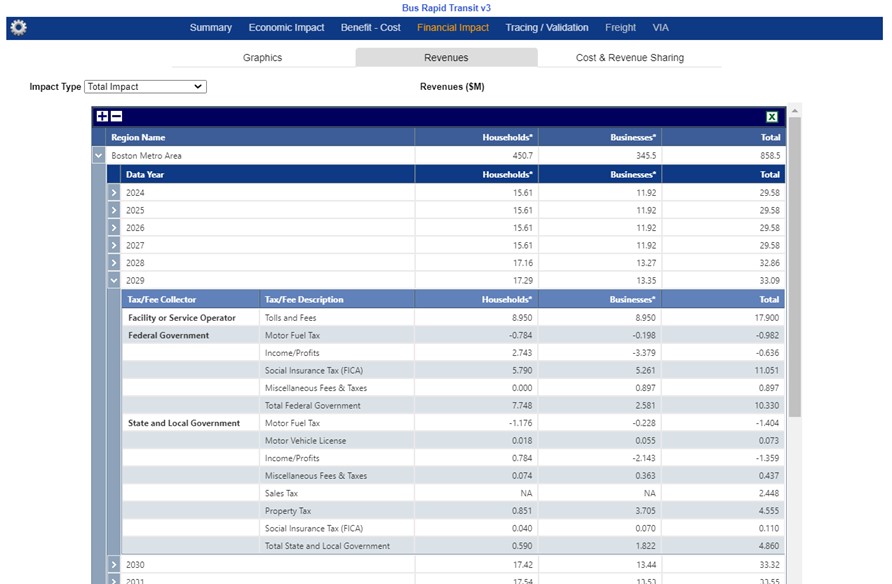
Note that Sales Tax is NA under the Household and Business disaggregate columns because the foundational IMPLAN data underlying TREDIS calculations does not provide the incidence split between the two entities.
Cost and Revenue Sharing
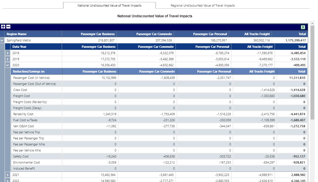
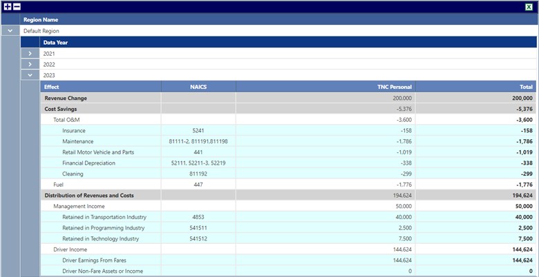
Of the $200,000, TNC management takes 25% of gross revenues, or $50,000 of revenues. Operating costs ($5,376) are then subtracted from the remainder, and finally Driver Income (via Driver Earnings from Fares) is what remains after operating costs. If the driver is operating at a personal loss for any reason, the improvement or worsening loss of this personal is shown in the line Driver Non-Fare Assets or Income, until the driver is no longer losing money by driving, after which it is reflected in income.
Results from this report inform the Costs Savings by Industry and Project Impacts by Industry reports. Total revenues to drivers and TNC companies are taken out of household or employer budgets.
The left side of the screen is a menu that allows you to move between comparison reports.
Multi-Criteria Compare – Projects Selection
When you first click on the Multi-Criteria Compare button, a new browser window opens to the tool. On the left are the top-level navigation tabs – Projects Selection, Overall Score, and Individual Metrics.The Projects tab on the Projects Selection page is the landing screen.
| Contract | Choose the Contract which contains the groups with the projects to be compared. |
| Group | Choose the Group which contains the projects to be compared. |
| Comparison Start Year/Comparison End Year | Choose the period of analysis; data outside of these years will be disregarded for the analysis. |
| Discount Rate | Select the discount rate to be used in the analysis. |
On the Metric Weighting tab, select the weights for each category of evaluation. The upper tier of weights entered must add to 100%. The bottom tier is only the relative weighting of factors within the larger Societal Benefits category. These are weighted just with integer weights, but there is no constraint on their sum.
Multi-Criteria Compare – Overall Score
The Overall Score screen has two tabs, the Table tab and the Chart tab. The Table tab displays the primary results of the analysis.
| Raw Metric Value | Raw values of component as calculated by TREDIS. |
| Scaled and Normalized | The values after normalization (which accounts for the cost of the project) and scaling (which puts the score on a continuum of scores between 0 and 100). For separate components of Societal Benefits, this is normalized and scaled relative to all the societal benefit components across all projects. For Societal Benefits row, this represents the components added then scaled among the totals. |
| Weight | Weights chosen in the Projects Selection screen. |
| Individual Score | The final score for the component. For Societal Benefits, this is scaled again to produce the total Individual Score for Societal Benefits. |
The Charts tab shows scoring data as a bar graph.
Multi-Criteria Compare – Individual Metrics
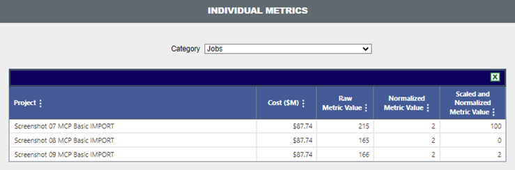
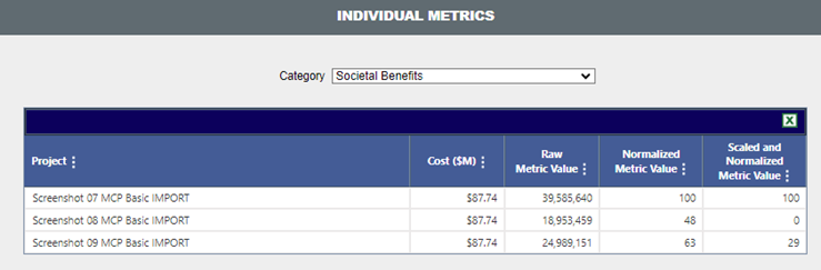
The individual metrics page allows you to perform tracing on the source of individual metrics. The Category dropdown allows you to choose the component of interest.
| Cost ($M) | Total discounted project cost. |
| Raw Metric Value | Values taken directly from project results. |
| Normalized Metric value | Values after normalization (where values are divided by cost to provide per-dollar metric). For Societal Benefits, reported Normalized Metric Value has already scaled to the value of the project with the highest Normalized Societal Benefits in order to be consistent with the overall scoring process. |
| Scaled and Normalized Metric Value | Values after normalization and scaling (where normalized values are adjusted to a score of 0 to 100 based on the minimum and maximum of the component). |
| TREDIS 6.0 User Manual | Return to Contents |
Multi Run & Summary Results
Overview
Some workflows, such as prioritization processes, require comparison of a substantial number of projects at the same time, often those sharing the same Construction and Operations periods. These could be imported in a single import, and, similarly, may be run and reported on in a single exported Excel workbook in a few clicks by using the Multi-Run & Summary Results functionality.
Accessing Multi-Run & Summary Results
From the Project page, click on the Group Options button at the bottom to reach the Group Options window. Select projects to run and export, keeping in mind they need to share at least Operations periods to be run through the Multi-Run & Summary Results function. Click the Multi-Run & Summary Results button to access the function.
Multi-Run & Summary Results Button with Projects Selected
Using the Window
The window that appears is used to control the running settings that will be used on all the projects being run and reported on.
In the top section, several options mirror those available in the regular Results Settings page. These include the following:
- Charge Interpolation
- Depreciation Type
- Safety Economic Impact
- Interpolation Method
- B/C Perspective
- Discount Rates
Multi-Run & Summary Results Window
Additionally, there are controls that are options that are specific to Multi-Run:
- Results Year. The year for which Long-Term Impacts are reported in the resulting output.
- Short-term Year. The years and type of reporting for which Short-Term Impacts are reported.
- Export File Name. Name of the file (with .xlsx appended) that will be produced.
- Confirmation Email. E-mail where the file will be sent. Not required.
- Rebuild Model. Rebuild the economic model. This is not commonly used and unlikely to be necessary unless you have been advised by TREDIS to use it.
When you have made your selections, click Run Analysis to launch the process and a status bar. For multiple projects, this process may take time.
When completed, a button for a direct download will appear if you do not wish to access via e-mail. Click Back to Project List to return to TREDIS.
Overview of Report
The resulting Excel file has three sheets.
- Read Me orients the user to the purpose of the workbook and includes version information.
- Summary Results Columns is the primary documentation for the report. Consult this for the most detailed explanation of results reported.
- Summary Results is the primary report.
Example Exported Workbook
| TREDIS 6.0 User Manual | Return to Contents |
Project Management - Create Project Backup
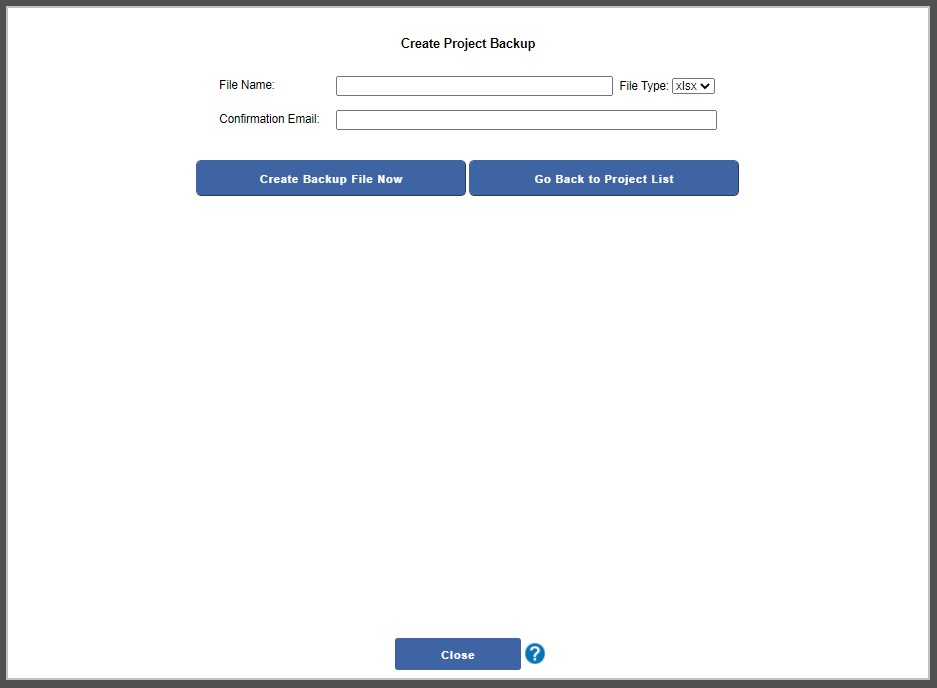
Enter a name for your Project Backup Spreadsheet and select the file type -
either .xlsx or .xls. Next provide your email address to be notified
when the backup process is completed.
Finally, press the Create Backup File Now button to start the process. When done, a download link will be provided and an email with a downlink if your email address was provided.
Finally, press the Create Backup File Now button to start the process. When done, a download link will be provided and an email with a downlink if your email address was provided.
| TREDIS 6.0 User Manual | Return to Contents |
Export Detailed Reports
TREDIS supports the exporting of a single Excel workbook with multiple sheets of results tables for a single analysis or multiple analyses. Users can create a workbook template to reuse across their projects, selecting which of the many reports they want to include in their workbook, as well as setting the options that affect the contents of those reports. Using the template, then the user can download all the reports at once.
This capability will now allow users to store all TREDIS results offline in case they are needed later at a time when they are no longer available in TREDIS.
Exporting for One vs. Multiple Projects
To export multiple reports for a single project, go to the Results page. The Multi-Report icon (a downward arrow) appears on the far right of the bar running along the width of the screen. This icon is available from any of the Results subpages.
The Multi-Run Icon
Clicking on this icon will open the Multi-Report Interface discussed below.
The same interface can be accessed for multiple projects so that you can export multiple reports for multiple projects. To access this functionality, start by clicking on the Group Options button on bottom of the Project page. The Group Options window will open.
Group Options Window with Projects Selected
From the Group Options window, select the projects to export reports for, and click the Export Detailed Results button to launch the Multi-Report Interface described below.
Running and Exporting Reports
Whether you are accessing it from the Results for a single project or from the Group Options window for multiple projects, the Multi-Report Interface will appear as below.
Multi-Report Interface
Reports are produced based on a template, so before TREDIS can produce a report, a template needs to be saved. For example, in the figure below, the reports for Total by Industry, Benefit – Cost Overview, Value of Benefits by Year, Cost Savings by Type, and Equity Context have been selected. In this example, the default settings (adjusted using dropdowns at the top) have been used.
The template has already been saved in figure above as Template Example for Release Note. Once you save a template, you will be able to use it whenever you access the Multi-Report Interface.
The name of the current template is provided in the pop-up that opens when you click Save As New Template. If you click Update Template, the settings for the selected template will be overwritten with your current selection.
You may need different batches of reports for different business processes, so TREDIS can save and reuse a template. Once a template is added, it can be accessed via the dropdown at the top of the interface, next to the Download File button.
Once you have saved a template, an Excel workbook based on this template can be prepared. Clicking Download File will start the file preparation process. When completed, the file will be downloaded to your device's Downloads folder or other default location.
Using the Export Workbook
The Excel workbook that you download will always include a Settings sheet, as seen below, that indicates what settings were applied to produce the results in the exported file.
Detailed Results Settings Tab
Each other worksheet represents a report. If you selected multiple projects to report on, separate projects are reported in the same sheet but are differentiated by the Project Name column, where the project name is given for the results. You can see the results for the first project selected in the Group Options interface. Scroll down further in a workbook to see results for the other projects selected, or add filters to the column headers to focus on specific projects or attributes.
Detailed Results Export Report Tabs
| TREDIS 6.0 User Manual | Return to Contents |
Timing
Project Timing
Construction Years and Operations Years in your project can be set by clicking on the
handle on the range of years and dragging left or right.
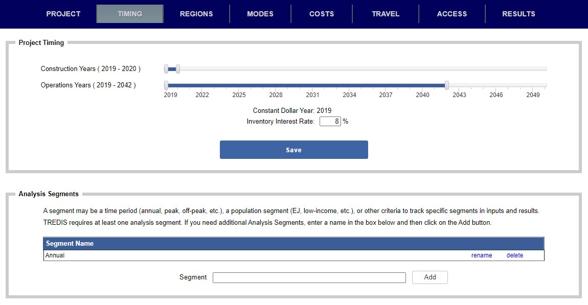
| Construction Years | The years when capital and design costs are modeled, for both spending and impacts |
| Operations Years | The years when recurring maintenance and operations costs and impacts are modeled |
Construction Years and Operations Years may overlap for as long as needed. For example, a
road widening might open a portion of the road to use mid-construction, at which point travel and operational costs
may be relevant while construction costs and impacts are still modeled as well.
| Constant Dollar Year | This value is now to the baseline economic data. For example, if the economic data is based on 2020, the constant dollar year is set at 2020. |
| Inventory Interest Rate | Enter this as a percentage representing the interest rate of private capital, which will be used for calculations of freight cost logistics. |
Analysis Segments
TREDIS allows you to divide your travel into segments to see how distinct groups of travelers affect the benefits
and impacts of the entire system. All segments are added together to make up the entire analysis, so any one
segment may not be a subset of another. Common uses of segments include differentiating periods of the day –
e.g. "AM Peak" and "PM Peak" segments – or demographic groups – e.g. "EJ population" and "Non-EJ population"
segments.
Each mode and region will be repeated on the Travel page for each segment defined, and some reports likewise give data on each segment separately (as well as a total of all segments). For example, if weekday Passenger Car - Personal travel makes up only a portion of traffic on weekdays, but nearly all of travel on the weekends, a "Weekday" segment and a "Weekend" segment will allow you to both enter and track the periods separately.
Keep in mind that activity in one segment doesn't affect activity in the other, even when divided into sequential segments, such as time of the day, so that a period labeled "AM Peak" will have no effect on another labeled "PM Peak".
Each mode and region will be repeated on the Travel page for each segment defined, and some reports likewise give data on each segment separately (as well as a total of all segments). For example, if weekday Passenger Car - Personal travel makes up only a portion of traffic on weekdays, but nearly all of travel on the weekends, a "Weekday" segment and a "Weekend" segment will allow you to both enter and track the periods separately.
Keep in mind that activity in one segment doesn't affect activity in the other, even when divided into sequential segments, such as time of the day, so that a period labeled "AM Peak" will have no effect on another labeled "PM Peak".
| TREDIS 6.0 User Manual | Return to Contents |
Regions
The Geographic Building Blocks of TREDIS Analysis
A TREDIS license is associated with specific counties, defined when the license is set up. Additionally, a license may have access to custom geographies, usually subcounty areas, if your license is set up to provide them. In any case, these are the basic building blocks used to build economic regional models, and each geography has its own detailed economic data, with metrics for hundreds of individual economic sectors.
Whether county-based or subcounty-based geographies are being used, they can be combined to form a Region in TREDIS. This is the smallest unit of geography for a TREDIS analysis, and any results reported by geographic area will be reported on by Region.
There are many reasons you might group smaller geographies into Regions. The following use cases represent some of the most common examples.
- You are interested in seeing the impacts of road improvements across the state, so you select all the counties in the state to make a single Region.
- You want to know the impact of bridge investments within the counties of a single MPO, but you also want to know if there are secondary economic impacts on the rest of the state. You create one Region with all the counties in the MPO, and another Region labeled "Rest of State" for all the other counties in the state.
- You want to know the impacts of a rural transit system on a single county, and you don't have any reason to look into impacts outside of that county. You select the county by itself to create a single Region.
A project must have a minimum of one Region, and each Region must be comprised of at least one geography (that is, at least one county or sub-county area). No two Regions may share the same geography, because allowing them to would mean you might inadvertantly double-count any impacts or benefits associated with a single county or sub-county area.
Using the Interface
To define and build the economic model you'll need for a TREDIS analysis, complete the following steps.Create Regions and Add Geographies
Aside from the default single Region that is provided whenever you create a project, you can add other regions with the Add Region button at top left. Each region is represented by a Region tile at the left, and each Region has a distinct color. In the screenshot, there are four Regions created, each colored on the map. Notice that some Regions have multiple counties associated with them, while one, "Worcester," is a single county.
In this example, the Regions have already been defined, and the counties that belong to them have already been selected. To do this in your own project, you can use one of two methods:
- Select the colored bar within the Region tile at left, and click on the map to add a county to the Region.
- Click on the dropdown menu within the Region tile and check boxes to add geographies to the Region.
In the screenshot, the first Region, named "Boston Area," is represented by the color red, and the counties associated with it are colored red on the map.
The last Region tile, for "Plymouth and Cape," has an open dropdown menu where the counties associated with it are already checked off, and other counties can be added.
On each Region tile, you can click the Rename button to relabel it, or Delete to get rid of the Region entirely.
Save the Definition of Regions
Once you are satisfied with the Regions you have defined, confirm your selections by clicking Save. Alternatively, you can click Revert Selection to get rid of any changes since your last save.
After you've saved the current definition, the Save button will appear gray to signify that the current definition is ready to be used to build the economic model. The Build Model button is now highlighted to indicate you are ready to build.
Build the Model
By clicking the Build Model button, you will launch the build process. This may take a few moments and you will see the progress indicator while it is proceeding. Once finished, the regular interface reappears and the button label changes from Build Model to Model Complete.
Storing and Recalling Regional Definitions
Regional Definitions may be reused between projects, allowing you to quickly select an existing definition of Regions -- one or many -- that you've previously stored, without having to click each county in the checkmark lists or on the map. Users may want to store definitions when they will be used frequently, especially across users or in a common business process.
What are Regional Definitions?
The defined Regions that are saved together when you click the Save button constitute a single Regional Definition in TREDIS. The economic model, which is built by TREDIS when you click Build Model, uses the Regional Definition to create the model used.
A single Regional Definition might involve a single region or multiple regions, but there is only one definition associated with any given TREDIS project. Each region may include one or more counties (or custom components such as subcounty areas). Like projects, Regional Definitions are stored at the contract level, so that other users that share a license may access the same Regional Definitions.
Regional Definition Controls
There are three controls with Regional Definitions:- The Store Current Definition button stores a definition.
- The Select Existing Definition dropdown selects and loads a definition previously stored.
- The Manage Definitions button opens an interface to view and delete stored definitions.
Storing a Definition
Click the Store Current Definition button to make the current Regional Definition available across projects and to other users.
A window prompt will ask you for a name to assign the Regional Definition so it can be referred to later. Once you enter a name and click Create, this Regional Definition will not be available in the Select Existing Definition dropdown to you and other users of your contract.
A Regional Definition must be saved before it can be stored. Storing a definition for later use is different from the effect of the Save button, which just confirms the use of the current definition for the TREDIS project you're currently working on. For an existing project, you will probably have already saved the Regional Definition, and the Save button will be greyed out, as in the figure below. For a new project, you will want to create a Regional Definition as you normally would and click Save. Once you have saved a Regional Definition, click the Store Current Definition button to store it.
Selecting an Existing Definition
For the TREDIS project you are currently working in, if you want to re-use a Regional Definition that has already been created and stored, click on the Select Existing Definition dropdown and select the Regional Definition from the list.
When you select a Regional Definition is from the dropdown, TREDIS will prompt you with a warning that whatever the current Regional Definition is -- whatever is being shown on-screen currently -- will be discarded to load the selected Regional Definition. Select Yes to continue and load the Regional Definition selected.
Managing Definitions
Definitions are stored at the contract level, which means they’re associated with the data year in the contract name. (For example, "TREDIS - 2021" would be for data from 2021.) Other users on the same contract can select and use them. To see all the Regional Definitions associated with the contract, click the Manage Definitions button to open a new window.
To hide definitions (so they don't appear in the Select Existing Definitions dropdown), click the Hide next to the name of the Regional Definition. When you're done changing the status of any Regional Definitions, click Update Hidden. To see definitions that were previously hidden, uncheck the boxes and click Update Hidden. To view the counties (or county equivalents) associated with a Regional Definition, click View on the row of the definition to open a window with that information.
Finally, if you are the creator of a Regional Definition, you may click Delete to do so. A prompt will confirm your choice before the Regional Definition is actually deleted. Other projects using the definition will not be affected analytically, but their Definition will be considered project-specific and unlabeled.
| TREDIS 6.0 User Manual | Return to Contents |
Modes
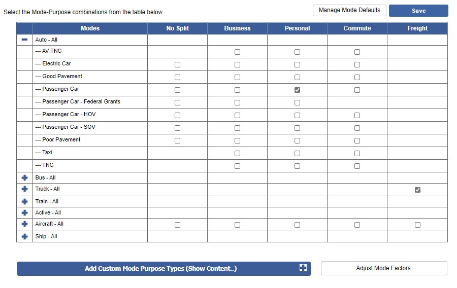
The next step in using TREDIS is to select the Modes of transportation and the
associated Purposes for your analysis. Using the check boxes contained on
this screen, simply check the box in the appropriate row and column.
The double downward arrow icon at the left side of a row indicates that there are detailed modes that may be chosen. Simply click on this icon to expand the list.
The double downward arrow icon at the left side of a row indicates that there are detailed modes that may be chosen. Simply click on this icon to expand the list.
|
The blue save button changes to orange to indicate a change has been made and the button needs to be pressed to save the change.
|
|
|
Pressing the Manage Modes button opens a new window that allows you to select
which modes to hide, uncluttering the Mode-Purpose table. This is
especially useful if your account has many custom modes.
|
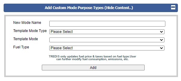
Add Custom Modes
Clicking on the Add Custom Mode Purpose Types bar will expand the screen to
allow you to create a new Mode/Purpose combination based on an existing one.
Provide a name for the new Mode, select a mode type from the drop down menu and
then select an existing mode to use as the template to create your new
Mode. Once you have created your new Mode, by clicking the Add button, you may
then update the fixed factors using the Manage Modes button at the top right of
this page.
Note: Beginning with TREDIS v5 custom modes are shared among
all users in your account. Once created they may not be deleted, however,
the creator may change the default characteristics of the custom mode.
Adjust Mode Factors
| Clicking on this button allows you to change the project defaults for the modes selected in the project. |
Only Mode/Purpose combinations selected
are displayed and the changes apply only for the current project. Once
you have finished entering your changes, please click the SAVE button
at the bottom of the screen. Use the CLOSE button to exit the screen.
| TREDIS 6.0 User Manual | Return to Contents |
Manage Modes
The Manage Modes screen allows you to view the default fixed factors for all default modes,
including those created by others in your account, and to update the values for any custom mode
that you created.
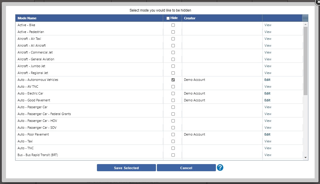
The screen shows all modes, both default and custom, with a checkbox that allows you to hide those modes that you do not need. For example, if you only deal with highway projects, then you can hide modes that are appropriate for air, marine, and rail, to reduce the clutter on your Modes screen.
In addition, you can see who created the custom modes in your account. In the picture below, the user logged in is the Demo Account and as creator of the custom mode (Auto - Electric Car) you may click on the edit link to change any of the default values for this mode. Anyone who uses this mode after the change will see the new values. Older projects will use the previous values.
Also, you are able to view the default values for custom modes created by others in your account but can not change any values.
The screen shows all modes, both default and custom, with a checkbox that allows you to hide those modes that you do not need. For example, if you only deal with highway projects, then you can hide modes that are appropriate for air, marine, and rail, to reduce the clutter on your Modes screen.
In addition, you can see who created the custom modes in your account. In the picture below, the user logged in is the Demo Account and as creator of the custom mode (Auto - Electric Car) you may click on the edit link to change any of the default values for this mode. Anyone who uses this mode after the change will see the new values. Older projects will use the previous values.
Also, you are able to view the default values for custom modes created by others in your account but can not change any values.
Once you have made your changes, click the Save Selected button to return to the Modes page.
You may also view the default values for the TREDIS Default modes or Custom modes
created by users in your account. If you are the owner of the Custom Mode, then you
are able to edit the default parameters.
Select the View link or Edit link as appropriate which will the Adjust Mode Factors screen.
Select the View link or Edit link as appropriate which will the Adjust Mode Factors screen.
| TREDIS 6.0 User Manual | Return to Contents |
Adjust Mode Factors
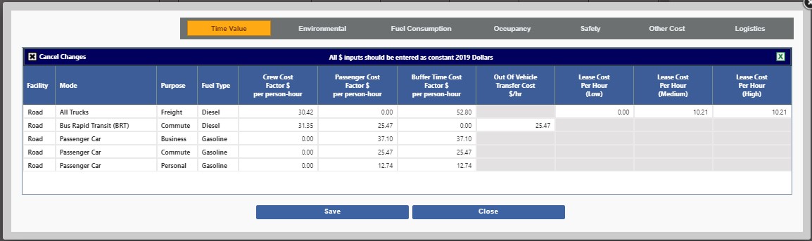
This screen allows you to change the default values within the current project for those modes which
have been selected. Once you have finished entering your changes, please click the SAVE button
at the bottom of the screen. Use the CLOSE button to exit the screen.
| Time Value | ||||||||||||||||
|
||||||||||||||||
| Environmental | ||||||||||||||||
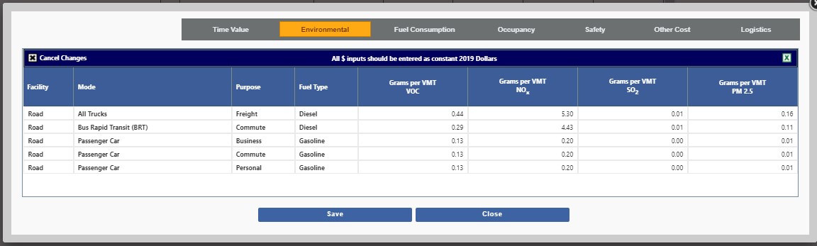
|
||||||||||||||||
| Fuel Consumption | ||||||||||||||||
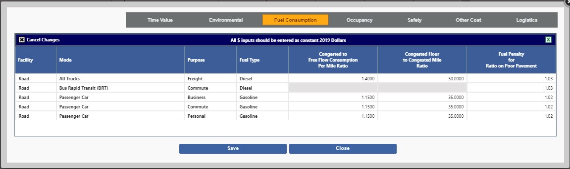
|
||||||||||||||||
| Occupancy | ||||||||||||||||
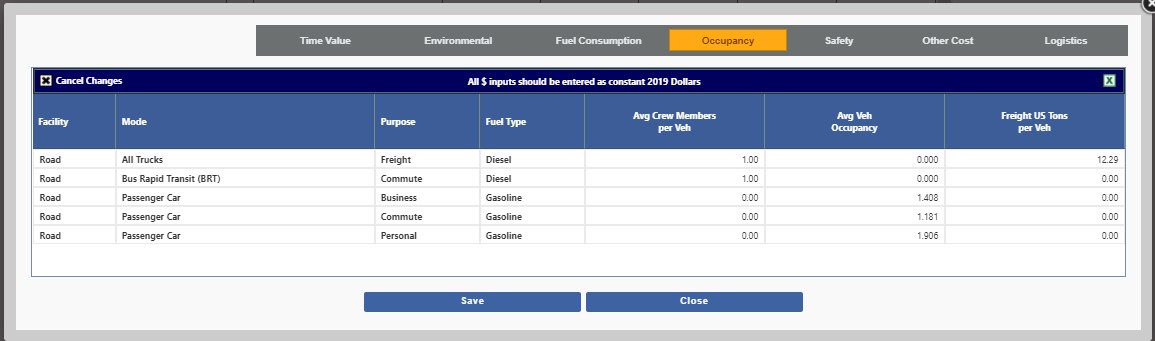
|
||||||||||||||||
| Safety | ||||||||||||||||
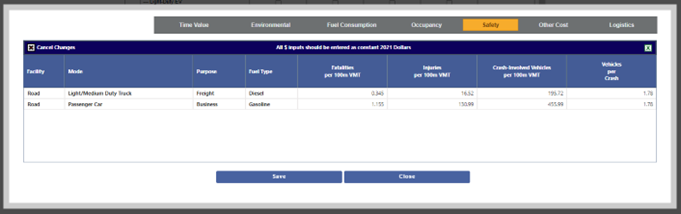
|
||||||||||||||||
| Other Costs | ||||||||||||||||
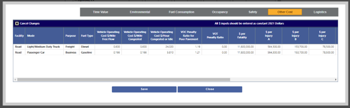
| ||||||||||||||||
| Logistics | ||||||||||||||||
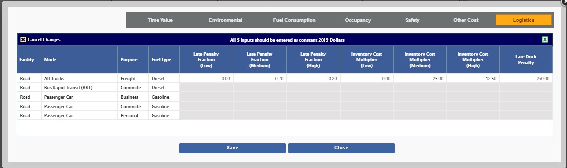
|
| TREDIS 6.0 User Manual | Return to Contents |
Costs
Users will often want to enter data to reflect one-time construction or improvement costs, as
well as on-going costs associated with operations and maintenance of facilities. The Costs
screen is where this data is entered.
Conceptually, the label "costs" reflects the use of these inputs in the Benefit-Cost Analysis, where the inputs are used in proportion to benefits, but keep in mind that for Economic Impact Analysis, costs are treated as spending that boosts economic activity.
TREDIS has two views of costs: Basic and Advanced.
Costs are defined by year, region, and facility. Each mode is associated with a facility. TREDIS differentiates the following facilities: Road, Passenger Rail, Freight Rail, Air and Marine.
The facilities available for input depend on the modes and purposes selected in the Modes Facility Based screen.
Note that all inputs are in millions. (The constant dollar year is set on the Timing screen.)
You can export the basic costs table to a spreadsheet and use the cut/copy/and paste functions to aid in your data entry.
The Save button will turn orange to remind you to click it if you make any changes. Red ticks on the boxes indicate values that have changed since the last change.
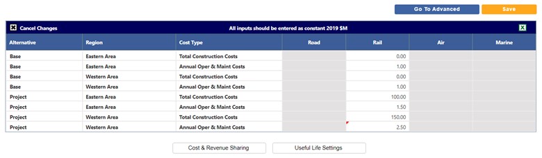
The following picture shows the Facility Based Project Cost screen for a two region model. This example is based on a rail project so only the Rail facility is shown. (Note: the Facility Based Project is the same as the standard project type in prior TREDIS versions.)
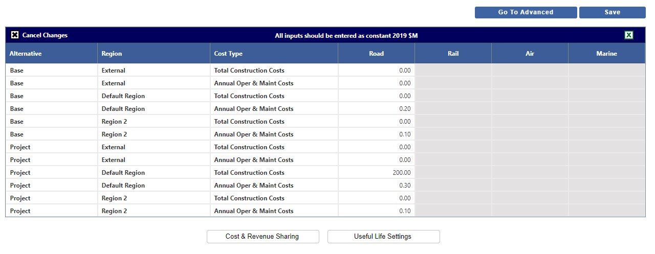
This next picture shows the O-D Based Project Type, also for a two region model. It should be noted that in this project there is a third region added called External to handle project costs outside the two main regions. This project only deals with trucks so only the Road facility is active.
Conceptually, the label "costs" reflects the use of these inputs in the Benefit-Cost Analysis, where the inputs are used in proportion to benefits, but keep in mind that for Economic Impact Analysis, costs are treated as spending that boosts economic activity.
TREDIS has two views of costs: Basic and Advanced.
Costs are defined by year, region, and facility. Each mode is associated with a facility. TREDIS differentiates the following facilities: Road, Passenger Rail, Freight Rail, Air and Marine.
The facilities available for input depend on the modes and purposes selected in the Modes Facility Based screen.
Basic View
TREDIS allows entries for Road, Rail, Air, and Marine facilities, showing only those that are applicable to the modes selected on the Modes screen.Note that all inputs are in millions. (The constant dollar year is set on the Timing screen.)
You can export the basic costs table to a spreadsheet and use the cut/copy/and paste functions to aid in your data entry.
The Save button will turn orange to remind you to click it if you make any changes. Red ticks on the boxes indicate values that have changed since the last change.
The following picture shows the Facility Based Project Cost screen for a two region model. This example is based on a rail project so only the Rail facility is shown. (Note: the Facility Based Project is the same as the standard project type in prior TREDIS versions.)
Basic Costs - Facility Based Project
This next picture shows the O-D Based Project Type, also for a two region model. It should be noted that in this project there is a third region added called External to handle project costs outside the two main regions. This project only deals with trucks so only the Road facility is active.
Basic Costs - O-D Based Project
Total Construction Costs
Each line for Total Construction Costs indicates the cost of the entire project’s investment, to be spread across all construction years (as designated in the Timing screen). The entire sum of the project investment (within the region and facility) is expressed in a single sum and represents a one-time total.Annual Oper & Maint Costs
Each line for Annual Operations and Maintenance Costs indicates costs that recur annually, whether for maintaining infrastructure, operating services, or other. These recur over every year in the Operations Years in the Timing screen.|
The blue Go To Advanced button next to the Save button will open the Advanced view of the Costs screen.
|
|
|
Click this button to open the Cost & Revenue Sharing window and allocate costs and
revenue between public and/or private entities.
|
|
|
Click this button to open the Useful Life Settings and change the useful life span of
facilities for your project.
|
|
|
Click this button to open the Quantities and Unit Costs window.
|
Advanced Costs
Using the Advanced view, you may enter detailed costs - Facility Based Project:
Advanced Costs - Facility Based Project
Using the Advanced view, you may enter detailed costs - O-D Based Project:
Advanced Costs - O-D Based Project
If there are many rows of inputs, you may want to filter by entering a filter argument in the fields below the column names, then clicking the filter button to choose a type of filter.
Notice that the Spending in Construction Years are available to input for every year of your Construction, and the Spending in Operations Years are available for input for every year of Operations, both set in the Timing screen.
Capital Costs Categories
Property Acquisition - Right-of-way purchases or easementsEngineering and Design - Soft costs of construction, including planning, analysis, legal, architectural, engineering, and design work.
Right of Way - Earthmoving, grading, drainage, and paving. For railroads, this includes all expenditures on the laying of rails; for airports, this includes runway construction.
Transport Structures - Construction of culverts, road bridges, flyovers, railroad bridges, and marine docks
Terminal - Operations offices, maintenance facilities, airport/bus/rail terminals, and storage buildings
Vehicles - Acquisition of rail cars and engines, ferries, airplanes, barges, or maintenance or service vehicles
Technology - Intelligent transportation systems (ITS), communications equipment, electric vehicle infrastructure
Operational Cost Categories
Operations and Services - For Road, Air, and Marine, operations costs for highway toll collection, systems operation, or incident managementPassenger Rail - Costs for operations for Passenger Rail, including systems operation, or incident management
Freight Rail - Costs for operations for Freight Rail, including systems operation, or incident management
Infrastructure and Rehabilitation - Crack repair, repaving, or vegetation control; also includes vehicle servicing.
Whenever there is a change to be saved, the blue SAVE button changes to Orange.
|
The blue Go To Basic button next to the Save button will open the Basic view of the Costs screen. Changing
to the Basic view will overwrite any changes you have made in the Advanced view.
Note: Changing to the Basic Mode will overwrite any changes
you have made in the Advanced Costs screen.
|
|
|
Click this button to open the Cost & Revenue Sharing window and allocate costs and revenue between public and/or private entities.
|
|
|
Click this button to open the Useful Life Settings and change the useful life span of facilities for your project.
|
|
|
Click this button to open the Quantities and Unit Costs window.
|
| TREDIS 6.0 User Manual | Return to Contents |
Cost and Revenue Sharing
The Cost and Revenue Sharing screen allows you to specify how project costs and revenue are distributed between
public and private agencies or organizations. For each type of project cost or revenue, the table shows the derived
amount (if applicable), then provides input variables to assign the share of the value on a fractional basis, between
the public sector and the private sector.
Project Costs
Project Costs
- Capital Costs ($m total for Construction Period) - the cost amount shown is derived
from the Start-up Cost Component input table
- Operations Costs ($m/yr for Operations Period) - the amount shown is derived from
the Annual Cost Components input table
- Maintenance Costs ($m/yr for Operations Period) - the amount shown is derived
from the Annual Cost Components input table
- Lease/Contract Costs ($m/yr for Operations Period) - the cost incurred by the
public or private agency to run the facility (the amount should be entered alongside the fractions public and private).
Project Revenues
- Toll Revenues ($m for Analysis Year) - the revenue amount is derived from
the Travel Demand Characteristics input table
- Lease/Contract Revenues ($m/yr for Operations Period) - the revenue
amount should be entered alongside the fraction public and private
Note: All values should be in terms of millions of dollars (or
local currency), leaving out the currency symbol.
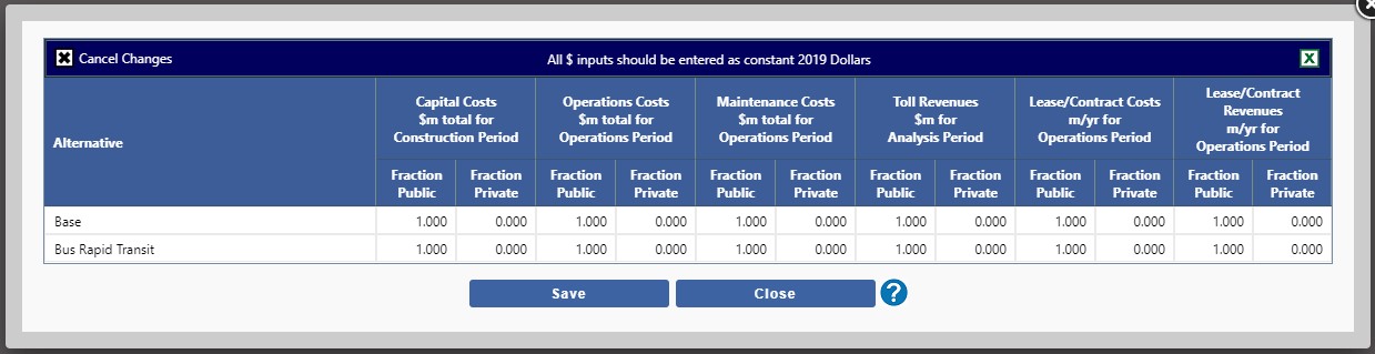
Note that, as with cost tables, inputs for the cost and revenue sharing table are
specified for all Alternatives (including no-build). The ultimate metrics (return
on investment, payback period) are based on the net differences between costs and
revenues for the case build vs. no-build.
You can export the basic costs
table to a spreadsheet and use the cut/copy/and paste functions to aid in your data entry.
The Save button will turn Orange to remind you to click it if you make
any changes.
- Toll Revenues ($m for Analysis Year) - the revenue amount is derived from the Travel Demand Characteristics input table
- Lease/Contract Revenues ($m/yr for Operations Period) - the revenue amount should be entered alongside the fraction public and private
Note: All values should be in terms of millions of dollars (or
local currency), leaving out the currency symbol.
Note that, as with cost tables, inputs for the cost and revenue sharing table are
specified for all Alternatives (including no-build). The ultimate metrics (return
on investment, payback period) are based on the net differences between costs and
revenues for the case build vs. no-build.
You can export the basic costs table to a spreadsheet and use the cut/copy/and paste functions to aid in your data entry.
The Save button will turn Orange to remind you to click it if you make any changes.
| TREDIS 6.0 User Manual | Return to Contents |
Useful Life Settings
The Useful Life Settings screen lets you change the average lifespan in years
for various elements for the four main facilities used by TREDIS:
- Right of Way - refers to roads, rail beds, runways, etc.
- Transport Structures - such as bridges and tunnels
- Buildings and Equipment - includes terminals and warehouses
- Vehicles - includes trucks, cars, trains, buses, aircraft, etc.
| TREDIS 6.0 User Manual | Return to Contents |
Quantities and Unit Costs
The Quantities and Unit Costs window allows an alternate way to enter capital costs for Construction Years. Once
these are entered, if any costs or units are not zero, all capital costs in Construction Year are taken from this window.
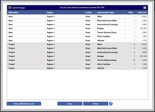
Once entered, total costs are distributed to appropriate categories across all construction years, and on the primary Costs page, the appropriate cells are greyed out (indicating they can’t be manually edited) and a notice at the top left indicates that Quantities and Unit Costs are being used for Construction capital costs.
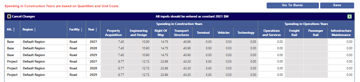
You can revert to manual entry by returning to the Quantities and Unit Costs window and clicking Clear All Unit Costs.
Once entered, total costs are distributed to appropriate categories across all construction years, and on the primary Costs page, the appropriate cells are greyed out (indicating they can’t be manually edited) and a notice at the top left indicates that Quantities and Unit Costs are being used for Construction capital costs.
You can revert to manual entry by returning to the Quantities and Unit Costs window and clicking Clear All Unit Costs.
| TREDIS 6.0 User Manual | Return to Contents |
Travel
The Travel page is where you enter data reflecting travel. This is an extensive page with multiple subtabs and buttons available to capture all the ways that travel can change between Base and Project alternatives. The primary use and functionality is described in the following subsections, with following sections detailing individual tabs and other interfaces that can be accessed.
Travel Data Entry and Tabs
The primary means for entering travel data in TREDIS is via a series of tabs, each of which has a data entry grid. Data can be manually typed, or it can be copy-pasted into the grid as if it were an Excel sheet. (If you do this, be careful, since you may be pasting into grayed out areas or outside of the grid.)
For Facility Based Projects, each row of data is defined by the Alternative, Region, Segment, Mode, and Purpose of the row, so the data entered only refer to that subset of travel. The rows where the Alternative is "Base" represent together the annual travel in the Base Alternative for the given Data Year (indicated on the upper right next to the Data Year control) – and the rows where Alternative is "Project" represent the annual travel in the Project alternative.
Travel Page with Data Input Grid Highlighted
For O-D Based Projects, the same is true, except Region is replaced by two fields: From Region (the origin region) and To Region (the destination region).
The primary data needed are entered on the Required Inputs tab. In TREDIS, economic benefits and impacts of the project are typically driven by differences in the Base and Project alternatives for metrics, especially those on the Required Inputs tab. As in the two rows above, the Region, Segment, Mode and Purpose columns all match values, but differ only by the Alternative. The differences in the Period VMT and Period VHT columns in those rows will often drive changes in the results, though this depends on the changes being modeled between Base and Project alternatives.
For private modes these data are primarily vehicle trips, vehicle miles traveled (VMT), and vehicle hours traveled (VHT). For transit vehicles and passenger aviation, these are passenger trips, passenger miles traveled (PMT), and passenger hours traveled (PHT) (though vehicle trips, miles, and hours can be entered for these other modes as well).
Other tabs are optional, but the same principle applies: Differences between the Base row and Project row for any combination of Period, Segment, Mode and Purpose reflect differences in the Base and Project alternatives. Data on other tabs may not be needed for your project if metrics are not expected to change or no localization is needed. See the Default Factors and Data Sources document for information on TREDIS defaults for many of these measures.
Note: For each analysis you do that is Facility Based, consider carefully the Flow tab. Lacking any project-specific information, the defaults for a new project assume all travel is within a region. This will not always be appropriate and leaving the defaults may result in overestimation of economic impacts for the region of interest. This is because any benefits for a trip that is 100% internal to the region are counted entirely for the region, whereas trips leaving or entering the region count for 50%, and through trips do not count at all for many purposes. This means it is easy to overestimate economic impacts if there is significant incoming, outgoing, or through traffic that is not accounted for on the Flow tab. For a BCA, the Region where benefits are enjoyed may not matter for the analysis, though if you are intending to differentiate benefits by Region it will make a difference.
Another condition to consider is if there are there are more passenger or freight-ton trips in the Project Alternative than the Base Alternative in a given year. This indicates inducted travel, and you should be aware of this and consider whether you will be accounting for the additional trips as induced. To do so, click the Trip Balancing button, which will automatically turn red if unbalanced trips are saved.
Travel Data Across Years
When first visiting the Travel page, the first Operations year is selected in the Data Year dropdown and the corresponding data is shown in the data entry matrix. In the years listed left-to-right, any year with data entered is in bold font. (The default is to consider this first Operations year as having been entered, since at least one year of data is needed for a TREDIS project.)
To delete entries for an entire year, select that year in the dropdown menu and then press the X icon to the right of the Data Year dropdown.
TREDIS will interpolate and extrapolate travel data for any years not entered. See the section describing the Results - Settings page for more information on choosing the interpolation method.
Travel Page with Data Year Controls Highlighted
Tabs on the Travel Page
The tabs running across the band navigate between sections for entering data.
Travel Page with Tabs Highlighted
Click on any of the grey tab names below to jump to the appropriate section. The Congestion-Reliability Input Method controls in the upper left of the figure above are used in conjunction with the Congestion tab – see that section for details.
Buttons on the Travel Page
There are 2 buttons at the top right of the screen and 5 running below the data entry grid serving various functions.
Travel Page with Buttons Highlighted
The Save button saves the current travel data shown on screen. For other functionality, click on any of the gray tabs below to jump to the appropriate section.
Facility-Based vs. O-D Based Projects
In the Project page, when a project is first created, its Travel Analysis Type can be set to be "Facility Based" or "O-D Based". In Facility Based projects, all fields on the tabs in the Travel page are entered by Region, starting with the required inputs such as vehicle trips, miles, and hours of travel. The proportions that are internal, incoming, outgoing, and through are indicated on the Flow tab. In the figure, travel is entered for each region.
Required Inputs for Facility Based Project
In contrast, in O-D Based projects, all fields on the tabs in the Travel page, including data on trips, miles and hours of travel, are entered on rows where each row is a combination of Regions, with a separate row for each combination of From Region and To Region. "External" in this case is counted as a Region in addition to any Regions defined on earlier on the Regions page.
Required Inputs for O-D Based Project
Travel – Required Inputs
The first tab is used to identify the number of vehicle (and in the case of transit modes, passenger) trips, distance traveled, and hours traveled.
Required Inputs Tab
Period Veh-Trips. The annual number of vehicle trips.
Period VMT. The annual vehicle distance traveled, in miles.
Period VHT. The annual vehicle travel, in hours, not including buffer time.
Transit Passenger Trips. Total annual passenger trips that is, the sum of all passenger trips.
Transit Passenger Miles. Total annual passenger distance traveled, in miles.
Transit Passenger Hours. Total annual passenger hours traveled.
Out of Vehicle Passenger Time. Total annual passenger hours spent to wait or connect.
Considerations
Depending on the travel modeling inputs you are translating to TREDIS inputs, you may need to convert from a daily figure to the annual figure required by TREDIS. For example, you may need convert "average weekday" values to annual values, possibly by multiplying them by 260 (52 weeks x 5 days/week). Consult the travel demand model specifications for details on what outputs represent in order to convert accurately. If multiple Segments are included and represent periods on a single day, make sure to annualize them all.
Transit modes and aviation modes allow you to enter passenger trips, miles, hours, and out-of-vehicle time directly. For all others, TREDIS will calculate these using vehicle metrics by multiplying by the occupancy rates. (For Freight purposes, this means vehicle metrics are multiplied by average freight tons in US tons). All occupancy rates are entered on the Occupancy tab.
Conversely, for transit and aviation modes, the occupancy rate is not entered but is can be found directly by dividing the passenger metric by the vehicle metric. Note that this may not be the same for trips, miles, and hours depending on the passenger usage profile.
Effects of Changes in Required Inputs
While projects may be complicated and many metrics may change between Base and Project alternatives, it can be useful to remember some basic relationships that will drive changes in costs, since cost changes ultimately impact all categories of results.
- Changes in vehicle or passenger trips will drive changes in per-trip charges or fees. This means that for many cases, changes in trips will not by themselves greatly change cost. However, a change in trips can indicate that you will need to indicate to TREDIS what share are induced trips. See documentation on Trip Balancing for more.
- Changes in VMT between Base and Project alternatives will drive changes in crash incidence, vehicle operating costs, fuel costs, and environmental costs.
- Changes in passenger hours traveled (either directly or via changes in VHT) will drive changes in passenger time cost and crew time cost.
- Changes in VHT for freight purposes will drive changes in freight logistics delay costs.
Travel – Occupancy
The Occupancy tab allows you to view and/or change the number of crew and passengers per vehicle as well as the freight capacities of modes that carry freight.
In the case of transit modes (bus and passenger rail for example), the average passenger occupancy rates are calculated from the values entered in the Required Inputs tab for vehicles and passengers, and may not be changed here. All values are initially set to the default values.
Note: You may only enter or update the values in those fields that are not gray.
Occupany Tab
Avg Crew Members per Veh. The average number of crew members per vehicle per trip. This has a default set at the mode-purpose level but can be changed by the user.
Avg Vehicle Occupancy. The average number of passengers (including the driver) per trip. For transit modes, such as passenger bus or rail, the value is calculated from the values on the Required Inputs tab as the ratio of Transit Passenger Trips/Period Veh-Trips. For freight modes, the field is not applicable and grayed-out.
Freight US Tons per Veh. The average number of US tons per vehicle per trip. This may be in a different unit if you are not using TREDIS in the US. For non-freight carrying modes, the field is not applicable and grayed-out.
Travel – Congestion
In TREDIS, the fraction congested is used to estimate how much vehicles are subject to extra costs from travelling in congested conditions, such as operating costs (e.g., wear-and-tear on brakes) and reduced fuel efficiency (from start-and-stop conditions). The concept of buffer time is used to represent time that is added to trips to account for unreliability. Unreliable travel times cause travelers to make early departures to buffer against potential delay. In TREDIS, buffer time represents the extra scheduling time in hours that ensures on-time arrivals for 95% of the trips.
Changes in congestion between your Base and Project alternatives will affect vehicle fuel efficiency. Changes in reliability (via buffer hours) affects time savings (both for private and crew travel), and freight logistics.
The metrics on the Congestion tab work in conjunction with the Congestion-Reliability Input Method control at the top of the Travel page.
Choosing the Congestion-Reliability Input Method
The Congestion-Reliability Input Method control has radio buttons and a dropdown, as shown in the figure below.
Use the radio buttons to select Both, Fraction Congested, or a reliability metric. Selecting the radio button next to Fraction Congested means you will enter only fraction congested. Selecting the radio button next to the reliability metric means you will only enter the reliability metric selected via the dropdown. Selecting Both means you will directly provide both.
Travel Page with Congestion-Reliability Preferences
In practical terms, this means that if you choose Fraction Congested here as the Congestion-Reliability Input Method, you will only be able to enter data in the Fraction Congested column in the matrix below, and the buffer hours that travelers add to their trips will be estimated based on the congestion. Likewise, if you select the third radio button and select Total Buffer Hours, TREDIS will only allow data entry in that column, and will later impute the fraction congested when performing the analysis. This option can be seen in the figure below.
Congestion Tab with Total Buffer Hours Chosen
Finally, selecting Both will mean TREDIS expects you to enter both the Fraction Congested and whichever reliability metric is selected. Anything not entered will be 0 by default.
After changing the Congestion-Reliability Input Method, the variables you can no longer enter will be greyed out in the entry matrix, the Save button will toggle to red to indicate there are unsaved changes. When you click Save, the stored values for the variable being imputed will be calculated based on your preferred variable, overwriting any previous values input when your preferences were set to Both.
When switching between reliability metrics, TREDIS automatically recalculates the appropriate values to be the equivalent of any data already entered.
Entering Congestion and Buffer Data
Fraction Congested. The fraction of all travel subject to congestion. For highway modes, it should be calculated as the fraction of VMT subject to a volume capacity greater than 0.9. The value represents a fraction, not a percent, so values must lie between 0 (no congestion) and 1 (pervasive congestion). Entering 0.3500 is valid, whereas entering 35 or 35% is not.
Buffer Hours per Trip. The number of hours of extra scheduling time needed to ensure on-time arrivals for 95% of the trips. For example, if a sample trip takes 30 minutes on average, but 1 out of every 20 days it takes 45 minutes, then the buffer time is 0.25 hours (or 15 minutes). This supports fractions of hours.
Buffer Time Index. The Total Buffer Hours as a fraction of total VHT. As an equation, Buffer Time Index = Total Buffer Hours / Vehicle Hours Traveled.
Total Buffer Hours. The total number of vehicle hours added as buffer. As an equation, Total Buffer Hours = Buffer Hours per Trip * Vehicle Trips.
NOTE: These variables and related factors are only used and calculated for private vehicles that use the Road facility.
Travel – Flow
For Facility-Based projects, the data inputs in the Flow tab indicate the fractional share of travel – measured by fraction of trips – taking place within, going out of, going into, or passing through the Region of the data row.
For O-D Based projects, all the columns in this tab will be grayed out, as they are not valid.
Internal Trips begin and end within the study region. All of their traveler benefits and all of the economic impacts are within the Region.
Incoming trips originate outside the region but end within it. Half of their traveler benefits and economic impacts are within the Region.
Outgoing trips originate within the region but end externally. Half of their traveler benefits and economic impacts are within the Region.
Through trips have both their origin and destinations outside the region, so that vehicles pass through the region (and use the travel facility) but do not stop there. None of their traveler benefits or economic impacts are within the Region.
In addition to determining where benefits and impacts are felt, for freight modes, the flow shares are used to match commodity costs to industries based on whether the commodities are being imported or exported. Incoming freight trips are matched to industries that use the commodities being shipped, whereas outgoing trips are matched to industries that produce the commodities being shipped. Internal trips are split between users and producers).
If the sum of the 4 shares in a row does not equal exactly 1.0000, you will get an error when you click Save and your changes will be lost for any rows where they don't sum correctly.
Review the following figure and the accompanying explanation to see how data input is to be interpreted:
Flow Tab
In the screenshot, the entered data for Passenger Car mean the following:
- 50% of trips take place within the Boston Region.
- 20% of trips end in Boston Region but originated externally.
- 20% of trips start in Boston Region but end externally.
- 10% of trips pass through Boston Region and don't stop.
Travel – Fuel
TREDIS includes federal and state fuel tax rates for various fuel types (gasoline, diesel, etc.) which may be overwritten as needed. Additionally, fuel efficiency can be changed.
Fuel Tab
Fuel Type. One of the following: Gasoline, Diesel, Electric, Aviation Fuel, Marine Fuel, or None. This field cannot be changed but shows the relevant fuel type for subsequent fields.
Fuel Cost. The cost in dollars per gallon or GGE (depending on the Fuel Type). This field is prepopulated with the cost for the fuel type shown, depending on the state. It includes both state and federal fuel taxes, which are shown in their respective columns in this table. The user may change fuel costs, but if the cost changes are due to changes in federal and/or state fuel taxes, then those values also need to be adjusted.
Federal Fuel Tax. The federal fuel tax per gallon or GGE (depending on the Fuel Type). The federal fuel tax is default to the current tax per gallon (or other unit of measure as appropriate for your country) and may be changed as desired. Defaults are provided for the different Fuel Types.
State Fuel Tax. The state fuel tax per gallon or GGE (depending on the Fuel Type). In a similar manner to federal fuel tax, this field allows you to override the state fuel tax rates.
Fuel Per Mile. Fuel used per mile, in gallons or GGE (depending on the Fuel Type).
Travel – Charges, Fees, Tolls
This tab is used to view and change various fees, taxes, and tolls on an average per vehicle basis.
Charges, Fees, Tolls Tab
Charge per Veh Mile. Average vehicle fees on a per mile basis, such as road user charges or mileage-based user fee.
Charges per Veh Trip. Average vehicle tolls and fees on a per trip basis. For transit modes, these tolls are assumed to be passed on directly to the passenger (and thus paid by the passenger as though it were a fee in addition to regular fares). If these charges would be paid by the agency to a road operator, rather than by the traveler to the road operator, they should not be recorded in Travel, but be included in the Costs page inputs as part of the operating expenses of the mode.
Charge Per Pass Trip. Average passenger fees per trip, such as for bus or train fares.
Charge Per Pass Mile. Average passenger per-mile fees, such as fares paid to some TNCs, taxis, and other on-demand transportation.
Travel – Safety
This tab is for safety incidents – fatalities, injuries, and vehicles associated with crashes – and adjustments.
Safety Tab
Fatalities per 100m VMT. Number of fatalities estimated for each 100 million miles traveled.
Injuries per 100m VMT Number of injuries of Unknown severity estimated for each 100 million miles traveled.
Crash-Involved Vehicles per 100m VMT. Number of vehicles damaged per 100 million vehicle miles travelled. This is only available when the Crash Entry Method (in the Preferences window) is set to Crash-Involved Vehicles.
Crashes per 100m VMT. Number of crashes per 100 million vehicle miles travelled. This is only available when the Crash Entry Method (in the Preferences window) is set to Crashes.
Considerations
When planning to entering safety data, consider whether you will use the rates method via the Safety tab (discussed here) or safety counts through the Safety Counts interface. Additionally, consider whether you want to get reports only on the social benefits of averted incidents or on social benefits and economic impacts. If you want to estimate economic impacts, you will need to select "Include" on the Safety Economic Impact radio buttons on the Results Settings page.
If a project adds distance traveled for both passenger car and bike/pedestrian travel, fatalities and injuries may be overestimated, since crash rates consider current average outcomes per mile. Defaults are provided for both as the modeled changes will typically be shifts between modes or within-mode analysis. The rates do not account for safety-in-numbers for non-occupants or the fact that many projects that increase bike/ped volumes will include safety improvements. When improving safety, consider using crash count inputs rather than default rates. Alternatively, crash rates can be zeroed out or reduced if increased bike/pedestrian trips should not be considered as facing increased crash risks beyond those represented by vehicular risks imposed on non-occupants.
Travel – Other
Other rates that are relevant to travel are set here.
Other Tab
Fraction of Pavement in Poor Condition. Fraction (0 to 1) of the road facility that is in "poor" condition. Penalty ratios are set on the Mode-Purpose level via the Modes page, via the Adjust Mode Factors button.
Fraction of Hours Traveled with Adjusted VOT. Fraction (0 to 1) of travel time whose value of time needs to be adjusted (depending on the mode, vehicle hours or in-vehicle passenger hours). Penalty ratios are set on the Mode-Purpose level via the Modes page, via the Adjust Mode Factors button.
Other Societal Benefits ($/VMT). Dollars per VMT that need to be added to the benefits, due to societal benefits that are not otherwise accounted for in TREDIS.
Other Societal Costs ($/VMT). Dollars per VMT that need to be subtracted from the benefits, due to societal benefits that are not otherwise accounted for in TREDIS.
Travel – Diagnostics
The Diagnostics window gives you a quick way to check performance data entered on the Travel page to confirm it represents the expected changes to support economic development.
For example, it may be assumed that the Project alternative (often the "Build" alternative) represents improved facilities that will allow users to go faster. The travel characteristics input into the Travel screen may not reflect that, though, and the Diagnostics page allows you to catch that earlier in your analysis workflow, before running the full project.
Changes Tab
Available for Facility Based and O-D Based projects. Changes by year for trips, miles per trip, and speed.
On this page, all changes are calculated as Project value minus Base value, unlike the reports under the Results page. This is because it's more intuitive to highlight increases as positives here, especially improvements in speed.
Diagnostics Page - Changes Tab
Time Series Tab
Available for O-D Based projects.
In the top half of the Time Series tab, Change in Passenger and Ton Hours Over Time, see the graph for total changes in Passenger and Ton Hours, summed by Purpose.
Diagnostics Page - Time Series Tab
Toggle whether purposes are shown by clicking on the purpose label at right in the legend.
In the bottom table, Regional Activity, you can see the total change by Origin and again by Destination. (Notice that both the Origin and Destination sections constitute the total universe of trips, so they cannot be added together, as this will double count all trips.) The year can be changed using the Data Year drop-down at top left.
Origin-Destination Freight and Passenger Tabs
The Origin-Destination Freight and Origin-Destination Passenger tabs show representations of ton-hours or passenger hours saved by direction of flow, with the origin region to the left and the destination right. Blue lines represent net savings (hours in project alternative are less than in base) and red line represent net increase (hours in project alternative are higher than in base). Hovering with your cursor over a line shows a pop-up detailing the project, base, and change values for the line, as in the figure. The Data Year is selected in the drop-down at top left.
Diagnostics Page - Origin-Destination Freight Tab
Travel – Safety Count Inputs
From the Travel page, clicking the Enter Safety Incidents Counts button at the bottom of the page will launch the Basic Incident Counts window.
Safety Counts Basic View
The Basic version of the interface only asks for incident counts by Region and Segment, so it is useful when you do not have the appropriate data to attribute fatalities, injuries, or crash-involved vehicle counts to specific modes.
Clicking on the Go To Advanced button will launch the Advanced Incident Counts window, where specific counts of incidents can be attributed to specific mode-purpose combinations. This is the level of detail used by societal benefit and economic impact calculations. The Advanced screen will automatically populate based on Basic and Rates inputs, but you may make subsequent adjustments if needed
Travel – Travel Cost Override
If you do not need TREDIS to calculate costs for you and already have total savings calculated, you may enter this data directly into TREDIS instead of entering travel data on the primary Travel page. This is an option for users with more comprehensive travel demand models. This option is not available for O-D Based Projects.
You can access this mode by clicking the Set to Override Mode button on the main Travel screen. Before proceeding, you will see a warning message telling you that any inputs you have entered on the main page are no longer being used.
Override Costs Tab
Total cost levels are entered on this page.
Passenger Cost. Total costs due to traveling passengers.
Crew Cost. Total crew costs (drivers and other workers), including benefits and other non-wage compensation.
Freight Cost. Total cost of moving of freight.
Reliability Cost. Total cost of reliability.
Veh Operating Cost. Total vehicle operating costs.
Toll Cost. Total of all tolls incurred for this mode.
Safety Cost. Total cost of safety incidents and crashes.
Environmental Cost. Total cost of emissions.
Override Flow Tab
Fractional flows are entered here to distribute the costs entered on the override Costs tab discussed directly above.
Fraction of Trips: Internal. The fraction of annual trips that begin and end within the Region.
Fraction of Trips: Incoming. The fraction of annual trips that begin outside the Region and have their destination in the Region.
Fraction of Trips: Outgoing. The fraction of annual trips that originating within the Region but terminate externally.
Fraction of Trips: Through. The fraction of annual trips that have both their origin and destinations outside the Region, where the vehicle passes through.
Travel Characteristics – Import Travel Data
If you want to load your travel data using a spreadsheet, access this interface by clicking on the Import Travel Data button at the bottom of the Travel screen. This opens a window that contains a link for downloading a template populated with your project name, earliest operations year, alternatives, region name(s), and modes and purposes. Use this template to enter travel data for the years you have data. Make sure the worksheet (tab) is labeled "Travel Demand Characteristics".
Once you have your data ready, click on the browse button to select your file, and then click the upload button. Your data for all years contained in the spreadsheet will be loaded into the system.
Remember that there must be a tab in the spreadsheet named "Travel Demand Characteristics" and do not add, delete, or reorder the spreadsheet columns.
| TREDIS 6.0 User Manual | Return to Contents |
Travel Characteristics - Trip Balancing
Overview and Context
When the total passenger trips for a given purpose rise between the Base and Project alternative, they are said to need "balancing" to indicate to TREDIS what portion of trips are induced by favorable transportation conditions."In-Model" trips represent trips that were undertaken in the Base alternative as well as the Project alternative, and which are assumed to have the same value for the people undertaking them.
"Induced" trips represent new trips undertaken in the Project alternative because travelers found new travel conditions that made a journey worthwhile when they were not in the Base alternative.
TREDIS assumes that the economic conditions are the same in any tested alternatives for a single scenario, so a different level of population and employment should not be the cause of trip "imbalance."
In some cases, a change in the number of trips between Base and Project alternatives is represented by in-model changes or a change in what inputs represent.
For example, if journeys made as one trip in the Base alternative are reported as two in the Project alternative – for instance, if a single bus trip now includes a transfer – the difference in the number of trips should be considered "in-model" because they don’t represent new journeys.
Another case where differences might be in-model are in mode switching. If some percentage of commuters that drive have switched to bus, the number of bus passenger trips is likely to have risen, but the difference is "in-model" since only the mode has changed.
Induced trips are journeys that were not available or feasible in the Base alternative. For example, if highway speeds have improved due to an additional lane in the Project alternative, more trips may be undertaken versus the number in the Base alternative because of the marginal cost in time.
Differences in trip counts due to technical constraints in a microsimulation model should be handled before TREDIS rather than by the Trip Balancing window.
The Trip Balancing Window
To launch the Trip Balancing window, click on the Trip Balancing button at the bottom of the Travel screen (see Figure 1 below).The Travel screen in Figure 1 shows increases in total trips between the Base alternative and the Project alternative. The occupancy rates (on the following tab) for all modes and purposes have been set to 1.0 to simplify the example, so that vehicle trips are equal to person trips.
The Trip Balancing button is orange because it needs attention.
Figure 1: Travel Screen
In Figure 1, the number of Business trips rises from the Base alternative to the Project alternative by a total of 500. Dividing by the number of Base alternative Business trips, TREDIS finds a 0.5 percent increase (500/10,000). Though there are two modes used for Commute – Electric Car and Passenger Car – they are considered together for purposes of Commute travel, which in total rises 1 percent (change in total commute trips divided by over total commute trips in Base alternative, or 100,000/10,000,000), while total Personal travel has risen by 2 percent.
In Figure 2, "50%" in the Overall % Induced column has been entered by the user to indicate that half of new traffic – any increase, regardless of purpose – is considered induced. This will be applied to each of the four modes shown in the other columns during Run Results.
Figure 2: Trip Balancing Overview
Figure 3 shows how, by toggling to Override by Purpose, the induced percentage can be set separately by year for each purpose (Business, Commute, Personal, and Freight), though in this case there is only 1 year.
Figure 3: : Override by Purpose
By selecting Detailed Yearly Override, you may reach the screen in Figure 4 showing the System Wide Imbalance tab, to see differences by region and period.
Figure 4: Detailed Yearly Override
In Figure 5, the Regional Imbalance Adjustments subtab opens a table where the percentage of induced activity can be set by purpose, by year, by region and by period (the most granular input structure).
Figure 5: Regional Imbalance Adjustments
| TREDIS 6.0 User Manual | Return to Contents |
Travel Characteristics - Freight Logistics
The Freight Logistics button opens a window for editing commodity mixes, commodity valuation, and key cost factors. Access this
functionality by clicking the Freight Logistics button at the bottom of the Travel screen:
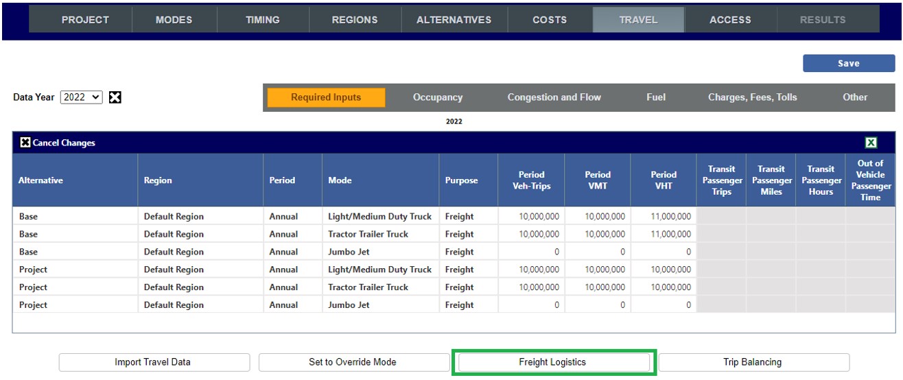
Commodity Mixes
On the Commodity Mixes tab, you can edit the commodity mix for your region across four different directions of travel.
Use the dropdown in the top left of the window to toggle between Internal, Incoming, Outgoing, and Through traffic.
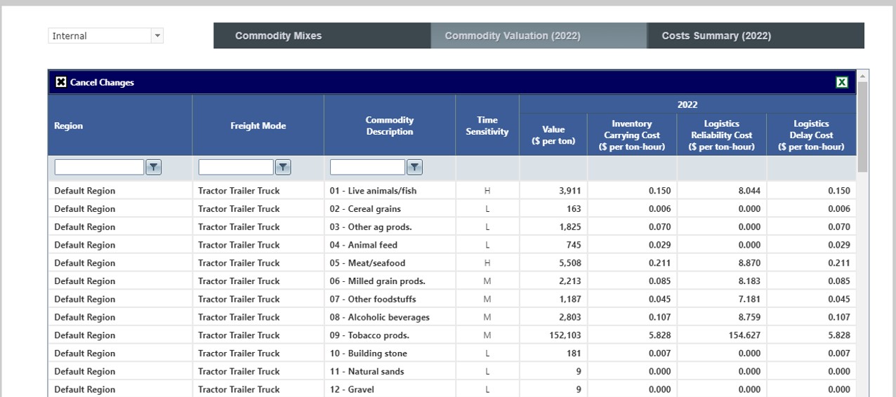
Costs Summary
Key cost factors are summarized here by mode using the commodity mix for the
region for the direction in the drop-down at top left. This data can be used to trace
results in the Cost Savings by Type report (in the Tracing/Validation group).
Figure 1: Accessing Freight Logistics
Commodity Mixes
On the Commodity Mixes tab, you can edit the commodity mix for your region across four different directions of travel.
Use the dropdown in the top left of the window to toggle between Internal, Incoming, Outgoing, and Through traffic.
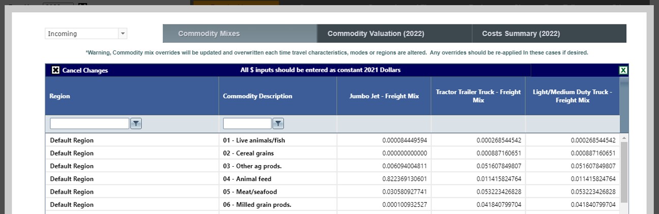 Figure 2: Commodity Mixes
Commodity Valuation
On the Commodity Valuation tab, you can edit the time sensitivity of different commodities if you’d like to apply
different assumptions than the TREDIS defaults.
| Inventory Carrying Cost | The $ per ton-hour of holding the inventory due to delays built into their scheduling and late docking fees applied because of trip scheduling |
| Logistics Reliability Cost | The $ per ton-hour of shipments that need to have buffer time |
| Logistics Delay Cost | The $ per ton-hour of logistics due to delays |
Figure 3: Commodity Valuation
Costs Summary
Key cost factors are summarized here by mode using the commodity mix for the
region for the direction in the drop-down at top left. This data can be used to trace
results in the Cost Savings by Type report (in the Tracing/Validation group).
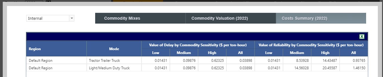 Figure 4: Cost Summary
| TREDIS 6.0 User Manual | Return to Contents |
Travel Characteristics – Safety Incident Counts
On the Other tab, users have the option of entering the rates of incidents – fatalities, injuries and crashes – per 100
vehicle miles travelled. There is an alternate way to enter directly these not as rates but as simple counts.
To access the count view, complete all other data inputs on the Travel page, including entering data for each year you have it for. This ensures that the Safety Incident Counts window will allow you to enter incident counts for those years.
To open the window, click the Enter Safety Incident Counts button.
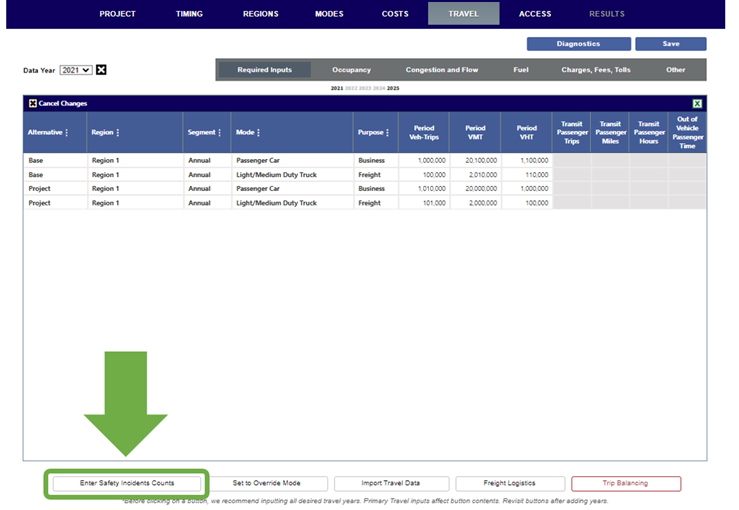
On the resulting Basic Safety Incidents Counts window, you can enter incident counts for KABCO severity of fatalities (or "K") and injuries ("A", "B", "C", and "O") where severity counts are known, for each alternative, region, and segment combination. Additionally, you may enter counts for severity "U" when injuries are estimated or observed but where the severity is unknown.
Depending on how you have set the Crash Entry Method in the Preferences window, either the Crash-Involved Vehicles or Crashes column will be available for input.
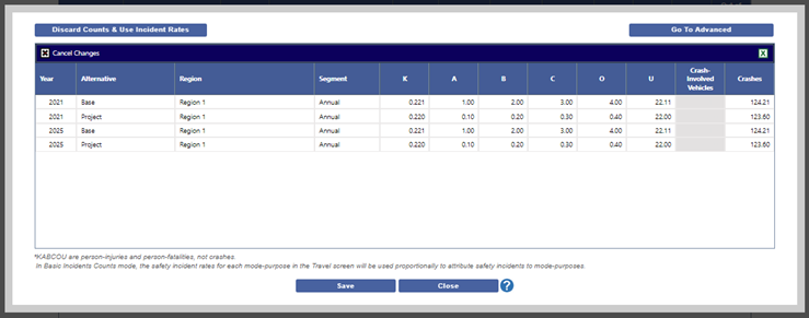
After clicking Save for any data entered, clicking the Go To Advanced button will take this data and attribute data to specific mode-purpose combinations and open the Advanced Safety Incidents Counts window.
Clicking Discard Counts and Use Incident Rates will discard the data entirely.
If you simply click Close, you will return to the Travel page and the project will use these Basic Incident Safety Counts unless you return to this window and click Discard Counts or Go To Advanced.
After clicking Save for any data entered, clicking the Go To Basic button to discard any Advanced Data entered and return to using the Basic Safety Incident Counts.
Clicking Discard Counts and Use Incident Rates will discard the data for both Basic and Advanced and return to using the default Incident Rates provided in the Travel page.
If you simply click Close, you will return to the Travel page and the project will use these Advanced Incident Safety Counts unless you return to this window and click Discard Counts or Go To Basic.
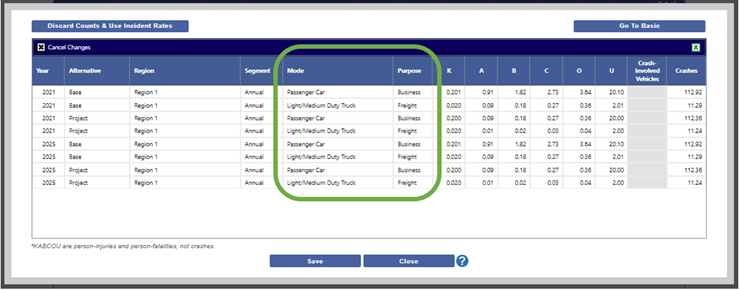
To access the count view, complete all other data inputs on the Travel page, including entering data for each year you have it for. This ensures that the Safety Incident Counts window will allow you to enter incident counts for those years.
To open the window, click the Enter Safety Incident Counts button.
Basic Safety Incident Counts
On the resulting Basic Safety Incidents Counts window, you can enter incident counts for KABCO severity of fatalities (or "K") and injuries ("A", "B", "C", and "O") where severity counts are known, for each alternative, region, and segment combination. Additionally, you may enter counts for severity "U" when injuries are estimated or observed but where the severity is unknown.
Depending on how you have set the Crash Entry Method in the Preferences window, either the Crash-Involved Vehicles or Crashes column will be available for input.
After clicking Save for any data entered, clicking the Go To Advanced button will take this data and attribute data to specific mode-purpose combinations and open the Advanced Safety Incidents Counts window.
Clicking Discard Counts and Use Incident Rates will discard the data entirely.
If you simply click Close, you will return to the Travel page and the project will use these Basic Incident Safety Counts unless you return to this window and click Discard Counts or Go To Advanced.
Advanced Safety Incident Counts
The Advanced Safety Incident Counts window is very similar to the Basic Safety Incident Counts window, but allows you to adjust counts for individual mode-purpose combinations where they are known. When first deployed, the window will pre-populate the counts based on any data entered in the Basic Safety Incident Counts window and the underlying Incident Rates that are given on the Travel page.After clicking Save for any data entered, clicking the Go To Basic button to discard any Advanced Data entered and return to using the Basic Safety Incident Counts.
Clicking Discard Counts and Use Incident Rates will discard the data for both Basic and Advanced and return to using the default Incident Rates provided in the Travel page.
If you simply click Close, you will return to the Travel page and the project will use these Advanced Incident Safety Counts unless you return to this window and click Discard Counts or Go To Basic.
| TREDIS 6.0 User Manual | Return to Contents |
Access
TREDIS estimates economic impacts stemming from spending (as entered on the Costs page) and travel improvements (entered on the Travel page).
Additionally, TREDIS can report on economic impacts beyond those spending and travel efficiency. The Access modules leverage additional user inputs to estimate economic impacts from two other major sources.
|
The Intercity Access module estimates how improvements in access on a county level can have economic impacts. Click on Intercity Access at left for more.
|
|||||||||||||||||
|
The Contingent Development module is for situations where new economic activity is contingent on a project being built, and the Project alternative should reflect the economic impacts of that activity.
Click on Contingent Development at left for more.
|
| TREDIS 6.0 User Manual | Return to Contents |
Access - Intercity Access
Overview
The primary benefits of transportation investments are often expressed in terms of time, cost, and/or safety for travelers moving between trip origins and destinations. However, there can be wider economic benefits when businesses gain access to broader labor, customer, and/or supplier markets. These effects increase productivity through what economists call agglomeration economies by increasing scale economies of production, matching of specialized worker skills to business needs, or matching of specialized business products or services to customer needs.
TREDIS recognizes three spatial ranges of market access effects.
- Local Market access focuses on urban-scale labor markets and consumer markets, which largely occur within a travel time range.
- Regional Market access focuses on same-day freight deliveries and same-day tourism, which largely occur within ranges of up to four hours each way. It can also generate —mega-region economic integration— benefits by connecting regions that have complementary industries.
- Access Times for Intermodal Connectivity focuses on the ability to access airports, rail terminals, and marine ports, which are gateways to broader national and international markets for people and freight.
Guidance
Not all projects or programs analyzed in TREDIS will have market access benefits. In general, they occur when there is a new or substantially improved network connection between population and business centers, or expanded modal options, or a shift to higher density development. A typical analysis will address at most just one or two of these categories.
Local Market — Corridor Investment: A corridor investment will connect a city to outlying areas, increasing the population within commuting range of the city and vice versa (connecting at least 15,000 people in outlying areas).
Regional Market — Corridor Investment: A corridor investment will enlarge the same-day travel and delivery market surrounding an employment center (adding at least 20,000 population or a business base of over 10,000 workers to that market).
Airport Access Time: A corridor investment will shorten average travel time from the city to a major airport (by at least 15 minutes).
Freight Rail Access Time: A corridor investment will shorten average travel time from the city to a TOFC/COFC terminal (by at least 10%).
Passenger Rail Access Time: A corridor investment will shorten average travel time to an intercity rail terminal (by at least 15 minutes).
Marine Port Access Time: A corridor investment will shorten average travel time from the city to a major marine port (by at least 10 minutes).
Regional Access Definition
The Regional Access Definition tab is the first step in defining access changes. The first Region defined on the Regions page is the selected region by default, but you can choose any Region. Each Region will have defaults for the selections, including the County of Focus and the intermodal access points.
These selections become relevant when you enter data on the Inputs tab, since the selections on the Regional Access Definition tab determine the baseline that all the data entered in Inputs is in reference to.
The map in the lower left corner shows all the Regions defined for the analysis. The main map shows just the current selections.
- Region Name: Select one of the regions you defined on the Regions page. All the subsequent selections depend on this selection.
- County of Focus: Select one of the counties within the Region. All the subsequent selections depend on this selection.
Airport Name, Freight Rail Terminal, Passenger Rail Terminal, and Port Name are all dropdowns (where multiple are available) to indicate the average time to reach the facility from closest to the most populous city in the county selected. Defaults are provided.
- Airport Name options are mid- to large airports.
- Freight Rail Terminal options are TOFC/COFC terminals.
- Passenger Rail Terminal options are terminals for passenger rail.
- Port Name options are marine ports.
The selected options are shown on the main map.
Once all your selections are made, click the Save and Reset Inputs button to update the Inputs tab with default data for your selections.
Inputs
The Inputs tab provides defaults in the Base alternative, repeated in the Project altnerative. You can change these or just change the expected time in the Project alternative.
There are three sections: Business Access to Population (Consumers and Labor Market Proxy), Business Access to Businesses (Employment), and Access Time (Minutes).
Access to Population and Businesses
Metrics. The columns under the Business Access to Population section represent the number of people that can reach the center of the county by car in the indicated amount of time. The Business Access to Businesses metrics are similar, except they measure the number of jobs. So, in the row for Boston Area, the value under Business Access to Population - 40 min column indicates the population that can reach the center point by car within 40 minutes, and the Business Access to Population - 4 hrs column indicates the number that can reach the center point by car within 4 hours. In the same row for Boston Area, Business Access to Businesses - 3 hrs, for example, indicates the number of jobs that can be reached from the center point by truck within 3 hours.
Significance. For Access to Population metrics, the population is taken to be a proxy for the potential labor market that can be employed by firms or consumer market that can be served by firms. With the goal of capturing consumer markets using typical variables available in models, we do not separately measure the number of workers in the calibration data or model application. An increase in the market size for a given distance metric between the Base and Project alternatives means there is a greater pool of talent available to employers, leading to better employment matching, or more access to consumers.
For Access to Business metrics, the measure of jobs indicates potential business relationships that can be leveraged for firms that provide or rely on other inputs.
Preparation. Access to Population and Access to Business both use access measures that normally require a network analysis, utilizing skim trees to identify all Traffic Analysis Zones (TAZs) reachable within various time thresholds from the central point. There are multiple time bands to enable impact decay functions, whereby local market access effects decay over a 40-minute to 1-hour range, while regional market access effects decay over a 1-4 hour range. See documentation for published research supporting these decay patterns.
Input. TREDIS automatically fills in values for the Base alternative, though the analyst may substitute their own inputs if available. Inputs for the Project alternative should match the Base alternative except where changes are to be expected.
Access Time
Metrics. The average time to the terminal or intermodal facility via truck or car from the central point.
Significance. Ports, terminals, and intermodal facilities are gateways to broader national and international markets for people and freight.
Preparation. The Access Time columns for airports, rail terminals and marine ports are normally calculated by a highway network model to calculate the shortest time path from each zone's designated city/town center.
Input. TREDIS automatically fills in values for the Base alternative, though the analyst may substitute their own inputs if available. Inputs for the Project alternative should match the Base alternative except where changes are to be expected.
| TREDIS 6.0 User Manual | Return to Contents |
Access ‐ Contingent Development
Overview
TREDIS provides an option for modeling Contingent Development, which is expected economic development that is contingent upon transportation investment. Industry impacts may be entered as sales (output) in millions of dollars or as employment as the total number of jobs added.
An example situation where Contingent Development would be useful is a warehouse that is being considered for development depending on whether access is improved. In the Project alternative, access is improved, and the warehouse is built, adding output and jobs to the local economy (whereas, in the Base alternative, the warehouse would not be built so no added output or jobs would be present).
This is useful because it allows further accounting within TREDIS (and thus within the Economic Impacts Analysis provided by TREDIS) for important economic events that are not directly reflected in improved travel efficiency (which would be reflected in inputs on the Travel page) or new construction or maintenance commitments (which would be reflected in inputs on the Costs page).
Entering Inputs
For a new project, on landing on the Contingent Development tab (under the Access page), you will see no records entered yet, as in the figure below. The box highlights the controls for choosing the Region and year where the contingent development would take place.
In this example, where a warehouse would be built contingent on the Project alternative being built, we enter 200 new jobs that the warehouse would support in the appropriate industry, then click the Save button to save this record.
If this new economic impact would last for the remainder of the Operations Period (defined on the Timing page), nothing more needs to be done. If another facility or change in the economic picture would occur in another year or region, enter that as a separate record.
For example, if the warehouse opening in 2035 (entered in the above example) with 200 jobs would expand in 2037 to support 400 jobs, create a record for 2037 and enter the data to model that.
In addition to commercial, retail, industrial and government sectors, the Contingent Development module also supports changes in households' "output" - here understood to be household income. Any change that would increase households' ability to spend could be input as a difference between the Base and Project values in the first "Industry" listed, Household Spending. Enter data in the Output ($M) to model any changes between the alternatives in households' income.
Interpolation
In cases where Contingent Development is entered for some years but not others, TREDIS interpolates and expands Contingent Development values to other years using rules similar to those used to expand and interpolate Travel characteristics. Trends of increasing or decreasing values are respected between and beyond the years input. This is intended to simplify data entry for those wanting to enter Contingent Development across multiple years where trends are observed but modeling has not been explicitly done.
Imputation between explicit zero values and non-zero values is allowed, as well as beyond the final input year, which is similar to how Travel data is expanded. When no zero value is explicitly set, all years until the first explicit entry are treated as zeros. Notably, this last rule is different from the method to expand Travel data across years, but is more intuitive for the behavior of Contingent Development, where discontinuous values are much more likely to be modeled. For instance, if a new factory, warehouse, or other source of employment opens in a given year, it might be very natural to model a large increase in the employment in that year that is a discontinuous jump from the year before.
| TREDIS 6.0 User Manual | Return to Contents |
Results
Before running your analysis to generate results, please review the default settings
and make adjustments as desired. Note, the analysis takes a few moments to
run. TREDIS saves your results and will show them without needing to run
the analysis again unless you change a value in the settings on this screen or go
back to your project and change other inputs.
After running your analysis, there are additional settings for running Freight Projects. Please view the TREDIS for Transearch or vFreight Help pages for setting up and running the appropriate Freight Analyses.
Description of Results Tabs
After running your analysis, there are additional settings for running Freight Projects. Please view the TREDIS for Transearch or vFreight Help pages for setting up and running the appropriate Freight Analyses.
The results navigation bar allows you to switch between report categories or go back to settings
to change the parameters used in the analysis.
Description of Results Tabs
 |
The Settings tab allows for defining the analysis parameters and running the analysis.
|
|
The Summary tab presents a graphical snapshot of your project results.
|
|
|
The Economic Impact tab provides details on the jobs, wages, business output, and value showing the economic
impact as a result of your project.
|
|
|
The Benefit-Cost tab provides details on the present value of the benefits
and costs, benefit-cost ratios, environmental factors,
performance metrics and the grant report for use in completing
TIGER applications.
|
|
|
The Financial Impact tab
contains information on tax impacts, cost & revenue sharing, and
investment return analyses.
|
|
|
The Tracing and Validation tab provides details supporting the other reports in the system.
|
|
|
For accounts with one of the freight options, this tab will provide analysis results. To view the
help for these options - click on one of the following two links:
|
| TREDIS 6.0 User Manual | Return to Contents |
Results – Settings
Before running your analysis to generate results, please review the default settings and make adjustments as desired. Note, the analysis takes a few moments to run. TREDIS saves your results and will show them without needing to run the analysis again unless you change a value in the settings on this screen or go back to your project and change other inputs.
After running your analysis, there are additional settings for running Freight Projects. Consult the sections on running with TREDIS with Transearch or TREDIS with vFreight for support on setting up and running the appropriate Freight Analyses. The results navigation bar allows you to switch between report categories or go back to settings to change the parameters used in the analysis.
Review and if desired change the default settings for running your analysis, then press the Run Analysis button. Anytime you make a chance to the settings or any inputs on the prior screens, you will need to rerun your analysis. Once finished, you are brought to the Summary screen.
Results - Settings Screen
Settings
Interpolation Method. This feature is used when TREDIS needs to compute travel characteristics values for year in which no user input is provided. The user may select from the dropdown menu using Compound Annual Growth rate or Straight Line Growth rate.
Charge Interpolation. Select None or Main Method. The None selection will use a step interpolation of charges. The Main Method will use the method chosen for Interpolation Method for charges.
Depreciation Type. Users may select whether to use a One-Time Project level depreciation method, where depreciation is computed for all project costs at once, or taking depreciation as an Annual Program, computing depreciation for each investment separately.
B/C Perspective. Select your analysis perspective: by Study Region or at a National level.
Safety Economic Impact. Select Include if you want the economic impact analysis to include impacts from changes in safety. Select Exclude otherwise. (The impacts from safety are calculated separately from safety benefits as reported in the Benefit-Cost Analysis, which are always reported.)
Buttons
Once you have selected your settings, press the Run Analysis button.
Run Analysis. Begin analysis of this project. The process will take a few moments and a popup window will appear to let you monitor progress. Once analysis is completed, you will not need to re-run the analysis unless you save new data on a previous page or on this Settings here.
Revert Settings. Reset any changes made so far to the Settings. This prevents the analysis from needing to be re-run if you inadvertently made changes to Settings that you don't need.
Costs of Emissions by Year. Opens a window allowing the update of default emissions costs for the project by the emissions type by year.
Costs of Emissions by Year
The costs of emissions by year can be changed from the defaults in a separate window that opens when you click the Costs of Emissions by Year button.
Costs of Emissions by Year Window
If changes are made that differ from the defaults, they will appear in red, as in the image below, where the user has already saved some changes from the defaults values. The Reset to Defaults button also appears.
Costs of Emissions by Year with Changes
| TREDIS 6.0 User Manual | Return to Contents |
Freight Analysis - Settings - Using Transearch
Running Freight projects involves two steps. The first deals with analyzing the
economic, benefit cost, and financial impacts, along with the tracing and validation
results. After this analysis has been completed, the Freight Analysis is run to provide
access to the freight results using the Transearch(R).
Before running your analysis to generate results, please review the default settings and make adjustments as desired. Note, the analysis takes a few moments to run. TREDIS saves your results and will show them without needing to run the analysis again unless you change a value in the settings on this screen or go back to your project and change other inputs.
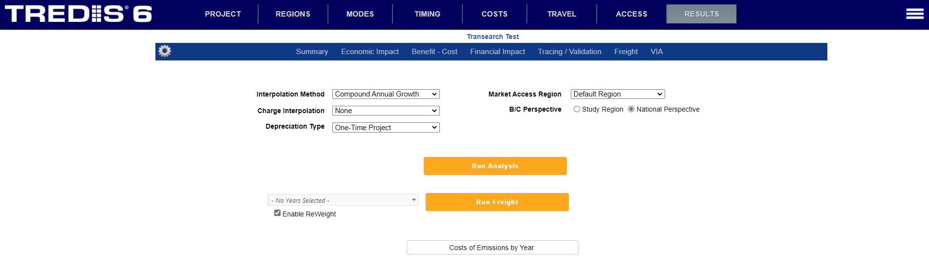
Before running your analysis to generate results, please review the default settings and make adjustments as desired. Note, the analysis takes a few moments to run. TREDIS saves your results and will show them without needing to run the analysis again unless you change a value in the settings on this screen or go back to your project and change other inputs.
For help on the standard settings, please refer to the help screen for settings by clicking on the gear icon:
| Area Type for Transearch commodity mix selection |
TREDIS needs to know if you are analyzing at the region, truck route, or rail route level when
assigning the commodity mix to the project. |
Once you have selected your settings, press the Run Analysis button. A popup indicator
will appear to let you monitor the analysis progress. The process will take a few minutes,
but once completed you will be able to select from the various tabs and quickly see your
results.
The first screen shown after the analysis is completed, is the summary tab which presents a story
of what changes were made to the transportation system and how they impact the economy:
View results or Run Freight analysis
You may now review the economic, benefit-cost, and financial impact results or you may go back to the settings screen - click on the gear icon, to run the freight analysis.You will notice that the Run Analysis button has turned blue indicating that the analysis has completed and the Run Freight is yellow indicating this analysis still needs to be run.
Please review and change the following settings for running you freight analysis:
| Area Type for Transearch freight run |
TREDIS needs to know if you want your freight analysis to consider the region, the specified
truck route, or specified rail route level when analyzing the freight portion of the project.
|
| Select years to analyze |
This drop down menu allows you to select the specific years for which you wish to
see results. You have the option to select all years or select specific years
by checking the box next to the desired year(s).
Note - the more years selected the longer this analysis will take to run.
|
| Enable ReWeight |
Check this box to have the system consider consumption and production levels of
trading partners relative to each other as part of the freight analysis.
|
Once you have specified the settings for the freight analysis, press the Run Freight button. Once completed, you will again be left on the summary screen, but will now have access to your freight results.
| TREDIS 6.0 User Manual | Return to Contents |
Freight Analysis - Settings - Using vFreight
Running Freight projects involves two steps. The first deals with analyzing the
economic, benefit cost, and financial impacts, along with the tracing and validation
results. After this analysis has been completed, the Freight Analysis is run to provide
access to the freight results using the vFreight data.
Before running your analysis to generate results, please review the default settings and make adjustments as desired. Note, the analysis takes a few moments to run. TREDIS saves your results and will show them without needing to run the analysis again unless you change a value in the settings on this screen or go back to your project and change other inputs.
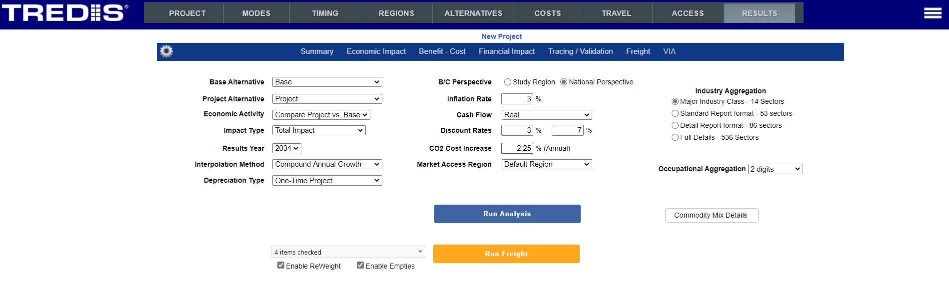
Before running your analysis to generate results, please review the default settings and make adjustments as desired. Note, the analysis takes a few moments to run. TREDIS saves your results and will show them without needing to run the analysis again unless you change a value in the settings on this screen or go back to your project and change other inputs.
For help on the standard settings, please refer to the help screen for settings by clicking on the gear icon:
Once you have selected your settings, press the Run Analysis button. A popup indicator
will appear to let you monitor the analysis progress. The process will take a few minutes,
but once completed you will be able to select from the various tabs and quickly see your
results.
The first screen shown after the analysis is completed, is the summary tab which presents a story
of what changes were made to the transportation system and how they impact the economy:
View results or Run Freight analysis
You may now review the economic, benefit-cost, and financial impact results or you may go back to the
settings screen - click on the gear icon, to run the freight analysis.
You will notice that the Run Analysis button has turned blue indicating that the analysis has
completed and the Run Freight is yellow indicating this analysis still needs to be run.
Please review and change the following settings for running you freight analysis:
| Select years to analyze |
This drop down menu allows you to select the specific years for which you wish to
see results. You have the option to select all years or select specific years
by checking the box next to the desired year(s).
Note - the more years selected the longer this analysis will take to run.
|
| Enable ReWeight |
Check this box to have the system consider consumption and production levels of
trading partners relative to each other as part of the freight analysis.
|
| Enable Empties |
Check this box to include the effects of empty/back haul vehicles in the analysis
|
Once you have specified the settings for the freight analysis, press the Run Freight button. Once completed, you will again be left on the summary screen, but will now have access to your freight results.
| TREDIS 6.0 User Manual | Return to Contents |
Results Summary
After a TREDIS analysis has finished processing, results are stored for the project and may be viewed. The Summary tab is the landing tab when accessing the Results page.
The Results Year dropdown menu allows you to select the year viewed on the Summary tab. The default is the last year of operations. The Impact Type dropdown allows you to filter the Economic Impact and Jobs by Year results. The default selection is Total Impact, meaning all sources combined, but the filter can be set to Construction, Operational, Contingent Development, or Market Access to identify specific sources.
Travel Changes
Bars indicate whether vehicle trips, miles traveled, and hours traveled rose or fell between the base and project alternatives.
For example, a rise of 2% in the Vehicle Miles Traveled (VMT) bar means there were more miles traveled in the Project alternative compared to the Base alternative. A drop of 7% in the Vehicle Hours Traveled (VHT) bar means there were fewer hours traveled in the Project alternative (which will translate to time savings).
Societal Benefit
Bars indicate the social benefits enjoyed in the Project alternative as compared to the Base alternative, broken out by traveler benefits, environmental social benefits, and wider economic benefits.
An increase of $300 million in traveler benefits means travelers were better off in the Project alternative, while a drop of $40 million in environmental and social benefits mean there were some disbenefits in the Project alternative.
Economic Impact
Bars indicate the increase in Gross Regional Product (GRP) in the Project case, by industry sector. For example, the blue bar at about $10 million indicates an increase in about that much GRP for the Project alternative (vs. the Base alternative).
Jobs by Year
The graph shows the number of extra jobs supported by the Project alternative over the Base alternative.
| TREDIS 6.0 User Manual | Return to Contents |
Results - Economic Impact
TREDIS allows you to filter your results using the drop down menu controls at the top of many of the economic impact results screens. Note that not all controls
appear on each results screen.
Graphics
The Economic Impact tab opens with a summary graphic showing for the sum of all regional jobs,
business output, value added, and wage income by year:
Impact Type |
The Impact type menu allows you to view the total impacts or filter the results to view only construction, operational, contingent development,
or market access impacts.
|
Economic Activity |
This control allows you to adjust the results view to look at the comparison between project versus base, the base results, or the
project results.
|
Industry Aggregation |
The Industry Aggregation menu allows you to adjust the industry details viewed in the results:
|
Occupational Aggregation |
The Occupational Aggregation menu allows you to adjust the details viewed in the results at the 2, 3, or 4 digit
occupational code level.
|
Graphics
The Economic Impact tab opens with a summary graphic showing for the sum of all regional jobs,
business output, value added, and wage income by year:
Interactive feature: Toggle on and off metrics to show by clicking on them in the legend.
Interactive feature: Click on a data point to reveal an industry disaggregation.
Clicking on this data point will open a graph showing by-industry breakdown of the metric (in this case, jobs). This view
begins with the top five industry sectors, which may be changed using the drop-down menu under the graph title.
Total by Industry
This interactive report presents the economic impacts of the project by year and for all regions in the project.
The number of industries is determined by the Results control panel option Industry Aggregation. The NAICS codes associated with them are provided.
Core metrics of Business Output, Value Added, and Labor Income are in millions.
Total by Occupation
This matrix provides a profile of the occupational type of jobs that are being generated by
the project. This type of information is important for economic developers. Much like industry, you can change the level of aggregation
reported with an option on the Results control panel, Occupational Aggregation. Occupation codes are SOC codes.
Core metrics of Business Output, Value Added, and Labor Income are in millions.
Quality of Jobs
The Quality of Jobs report shows characteristics of the jobs created by the project, with details categorizing occupations by wage
criteria (High Wage, Medium Wage, Low Wage) and whether jobs in in each category are growing or not.
By clicking on the tabs above the graph, you can toggle between viewing Quality of Jobs as a chart or table.
- Not Growing means an occupation is projected to grow less than 0.5% annually.
- Growing, Unstable means an occupation is growing but turnover is relatively high.
- Growing, Stable means an occupation have relatively less turnover.
The growth benchmark of 0.5% annual growth is set by research into the projected 2018-2028 growth trends. For context,
no-growth occupations employed 36.1 million workers in 2018.
The stability benchmark is set around a premium of 25% more openings per year than the average occupation (after
accounting for openings occurring from overall growth). The average turnover has been calculated as 11.7%, so the
threshold for being considered unstable is 14.6% turnover. Higher than this threshold is considered unstable, and below
is considered stable.
Productivity
Productivity shows changes in Value Added across industries.
- Direct Productivity Impact displays millions of dollars of net revenue change.
- Total Labor Productivity is defined as Value Added per worker.
- Total Labor Productivity Relative to US Average compares these figures to national trends.
Value Added per worker grows as cost savings is retained as profit or is spent on additional Labor Income which increases Value
Added. These gains are calculated into weighted average values for aggregated industries (such as 3-digit NAICS). This may increase
or decrease actual productivity depending on the 1) mix of industries, 2) their associated productivity, and 3) the gains in productivity
due to travel cost savings.
Competitiveness
The first three columns show the input intensity show the ratio of output per unit cost of labor, capital, and transportation in comparison to
the national average. The fourth column lists the Relative Labor Cost per worker and fifth column shows the Output Growth rate of the
previous 5 years compared to the U.S. average.
Supply/Demand
In addition to the regional and yearly breakdowns, this report shows industry aggregations based on the Industry Aggregation option in the Results control panel.
- Demand (Gross Purchases) shows a total, the amount produced and consumed with the region,
and the portion of the total imported.
- Production (Gross Sales) shows a total, the amount produced and consumed with the region,
and the portion of the total imported.
Pop / Labor
TREDIS calculates the expected impacts on population and the labor force within the study
region(s) by year and by industry aggregation.
For each region-year report, three panes are available:
- Labor Statistics is base information about jobs, labor force, and wages.
- Population Statistics is base demographics about population and households.
- Building Occupancy Needs shows the change (Alternative – Base Case) in multiple categories.
For more information please refer to the TREDIS 5 Dynamic Regional Economic Simulation Model document in User Documentation.
The number of industries is determined by the Results control panel option Industry Aggregation. The NAICS codes associated with them are provided.
Core metrics of Business Output, Value Added, and Labor Income are in millions.
This matrix provides a profile of the occupational type of jobs that are being generated by
the project. This type of information is important for economic developers. Much like industry, you can change the level of aggregation
reported with an option on the Results control panel, Occupational Aggregation. Occupation codes are SOC codes.
Core metrics of Business Output, Value Added, and Labor Income are in millions.
Core metrics of Business Output, Value Added, and Labor Income are in millions.
Quality of Jobs
The Quality of Jobs report shows characteristics of the jobs created by the project, with details categorizing occupations by wage
criteria (High Wage, Medium Wage, Low Wage) and whether jobs in in each category are growing or not.
By clicking on the tabs above the graph, you can toggle between viewing Quality of Jobs as a chart or table.
- Not Growing means an occupation is projected to grow less than 0.5% annually.
- Growing, Unstable means an occupation is growing but turnover is relatively high.
- Growing, Stable means an occupation have relatively less turnover.
The growth benchmark of 0.5% annual growth is set by research into the projected 2018-2028 growth trends. For context,
no-growth occupations employed 36.1 million workers in 2018.
The stability benchmark is set around a premium of 25% more openings per year than the average occupation (after
accounting for openings occurring from overall growth). The average turnover has been calculated as 11.7%, so the
threshold for being considered unstable is 14.6% turnover. Higher than this threshold is considered unstable, and below
is considered stable.
Productivity
Productivity shows changes in Value Added across industries.
- Direct Productivity Impact displays millions of dollars of net revenue change.
- Total Labor Productivity is defined as Value Added per worker.
- Total Labor Productivity Relative to US Average compares these figures to national trends.
Value Added per worker grows as cost savings is retained as profit or is spent on additional Labor Income which increases Value
Added. These gains are calculated into weighted average values for aggregated industries (such as 3-digit NAICS). This may increase
or decrease actual productivity depending on the 1) mix of industries, 2) their associated productivity, and 3) the gains in productivity
due to travel cost savings.
Competitiveness
The first three columns show the input intensity show the ratio of output per unit cost of labor, capital, and transportation in comparison to
the national average. The fourth column lists the Relative Labor Cost per worker and fifth column shows the Output Growth rate of the
previous 5 years compared to the U.S. average.
Supply/Demand
In addition to the regional and yearly breakdowns, this report shows industry aggregations based on the Industry Aggregation option in the Results control panel.
- Demand (Gross Purchases) shows a total, the amount produced and consumed with the region,
and the portion of the total imported.
- Production (Gross Sales) shows a total, the amount produced and consumed with the region,
and the portion of the total imported.
Pop / Labor
TREDIS calculates the expected impacts on population and the labor force within the study
region(s) by year and by industry aggregation.
For each region-year report, three panes are available:
- Labor Statistics is base information about jobs, labor force, and wages.
- Population Statistics is base demographics about population and households.
- Building Occupancy Needs shows the change (Alternative – Base Case) in multiple categories.
For more information please refer to the TREDIS 5 Dynamic Regional Economic Simulation Model document in User Documentation.
By clicking on the tabs above the graph, you can toggle between viewing Quality of Jobs as a chart or table.
- Not Growing means an occupation is projected to grow less than 0.5% annually.
- Growing, Unstable means an occupation is growing but turnover is relatively high.
- Growing, Stable means an occupation have relatively less turnover.
The stability benchmark is set around a premium of 25% more openings per year than the average occupation (after accounting for openings occurring from overall growth). The average turnover has been calculated as 11.7%, so the threshold for being considered unstable is 14.6% turnover. Higher than this threshold is considered unstable, and below is considered stable.
Productivity shows changes in Value Added across industries.
- Direct Productivity Impact displays millions of dollars of net revenue change.
- Total Labor Productivity is defined as Value Added per worker.
- Total Labor Productivity Relative to US Average compares these figures to national trends.
Value Added per worker grows as cost savings is retained as profit or is spent on additional Labor Income which increases Value
Added. These gains are calculated into weighted average values for aggregated industries (such as 3-digit NAICS). This may increase
or decrease actual productivity depending on the 1) mix of industries, 2) their associated productivity, and 3) the gains in productivity
due to travel cost savings.
Competitiveness
The first three columns show the input intensity show the ratio of output per unit cost of labor, capital, and transportation in comparison to
the national average. The fourth column lists the Relative Labor Cost per worker and fifth column shows the Output Growth rate of the
previous 5 years compared to the U.S. average.
Supply/Demand
In addition to the regional and yearly breakdowns, this report shows industry aggregations based on the Industry Aggregation option in the Results control panel.
- Demand (Gross Purchases) shows a total, the amount produced and consumed with the region,
and the portion of the total imported.
- Production (Gross Sales) shows a total, the amount produced and consumed with the region,
and the portion of the total imported.
Pop / Labor
TREDIS calculates the expected impacts on population and the labor force within the study
region(s) by year and by industry aggregation.
For each region-year report, three panes are available:
- Labor Statistics is base information about jobs, labor force, and wages.
- Population Statistics is base demographics about population and households.
- Building Occupancy Needs shows the change (Alternative – Base Case) in multiple categories.
For more information please refer to the TREDIS 5 Dynamic Regional Economic Simulation Model document in User Documentation.
- Demand (Gross Purchases) shows a total, the amount produced and consumed with the region, and the portion of the total imported.
- Production (Gross Sales) shows a total, the amount produced and consumed with the region, and the portion of the total imported.
Pop / Labor
TREDIS calculates the expected impacts on population and the labor force within the study
region(s) by year and by industry aggregation.
For each region-year report, three panes are available:
- Labor Statistics is base information about jobs, labor force, and wages.
- Population Statistics is base demographics about population and households.
- Building Occupancy Needs shows the change (Alternative – Base Case) in multiple categories.
For more information please refer to the TREDIS 5 Dynamic Regional Economic Simulation Model document in User Documentation.
| TREDIS 6.0 User Manual | Return to Contents |
Results - Benefit-Cost
Graphics
The Benefit-Cost tab starts on the Graphics sub-tab, which shows a chart for the different components of the Benefit-Cost analysis.The Graphics and Benefit-Cost tabs present three different groupings of benefits with the Societal benefit encompassing total benefits. The following sections explain the benefit groupings and their components in detail.
Traveler Benefit
Traveler Benefit represents benefits to travelers and the businesses that employee them. It is the most narrowly focused of the 3 types of benefit tabulations.- Business Time & Reliability Cost
- Value of Personal Time & Reliability
- Consumer Surplus
- Vehicle Operating Costs
- Safety Costs
User Benefit
User Benefit represents benefits to travelers (and their employers) but also includes Logistics Costs, which represent the cost of managing freight.Societal Benefit
The Societal Benefit tabulation includes all of the traveler and user benefits, but also incorporates externalities. The full list of categories considered is as follows:- Business Time & Reliability Cost (from Traveler Benefit)
- Value of Personal Time & Reliability (from Traveler Benefit)
- Consumer Surplus (from Traveler Benefit)
- Vehicle Operating Costs (from Traveler Benefit)
- Safety Costs (from Traveler Benefit)
- Logistics Costs (from User Benefit)
- Business Productivity (unique to Societal Benefit)
- Social (including Environmental benefits/disbenefits) (unique to Societal Benefit)
Costs
Cost categories in TREDIS represent direct, monetized costs of designing, building, and maintaining infrastructure, summarized in the following categories:- Construction
- Operations & Maintenance
- Residual
Using the Graphics Tab
Because Traveler Benefit, User Benefit, and Societal Benefit cover similar categories, you may choose to toggle off one or two benefit bars of the tabulations if they aren’t relevant to your analysis.Interactive feature: Toggle on and off metrics by clicking on them in the legend. For example, User Benefit and Societal Benefit may be toggled off to see only Traveler Benefit and Costs.
Interactive feature: Click on a Benefit bar reveal a disaggregation by category. Clicking on the Traveler Benefit bar above, for example, shows the breakdown between categories:
Interactive feature: Click on the Costs bar to reveal a disaggregation by Costs categories:
Interactive feature: Update the Discount Rate and click Refresh to change the discount rate for all measures.
Benefit-Cost Overview
The Benefit-Cost Overview tab shows a tabulation of Benefit-Cost Analysis results for the discount rates selected in Results settings. As with all similar tables, clicking the blue arrow on the left expands the selected category.All values are in present values (discounted) terms, in millions of dollars.
See the Benefit-Cost FAQ for details on the signs of Benefit and Cost categories.
Present Value of Benefits Stream
This table drills down into the various categories of net benefits that a project or policy change can bring about.- Benefit Stream – Travel Benefits These benefits are associated with travelers and traveling, including categories for time savings and safety as well as vehicle operating costs.
- Benefit Stream – Environmental and Social Benefits These benefits are associated with environmental effects, greenhouse gas production, and other social benefits as defined by user.
- Benefit Stream – Wider Economic Benefits These are benefits associated strictly with business productivity, labor market participation, and logistics and supply chain savings.
- Benefit Stream – Transfer Benefit Effects. These benefits specifically deal with adjustments due to fees, for example fees, tolls, or other user charges.
Present Value of Costs Stream
The next section addresses the Present Value of Cost Stream, detailing Project Costs and Cost Adjustments.- Costs Stream – Project Costs These costs represent actual design, capital spending, and operational and ongoing maintenance costs associated with the project.
- Costs Stream – Cost Adjustments These costs are often residual values of capital, following its use for the project.
Net Benefit
Three kinds of BCA analysis are calculated here.- Transportation System Efficiency: Traveler Benefits Only Traveler Benefit minus Present Value of Costs Stream
- Traditional BCA: Traveler Benefit + Economic Benefits Traveler Benefit plus Wider Economic Benefit minus Present Value of Costs Stream
- Full Societal BCA: All Benefits Categories Traveler Benefit plus Wider Economic Benefit plus Environmental and Social Benefit, minus Present Value of Costs Stream.
- Benefit Cost Ratio See the section above for the meaning of Transportation System Efficiency, Traditional BCA, and Full Societal BCA. Here, those benefit categories are divided by the Present Value of Costs Stream for a ratio.
Value of Benefits
This tab shows the benefit values by type by year for two different discount rates or undiscounted. These categories are the same as presented in the Graphics page, but grouped A through E, depending on the type and whether the benefit is monetized or non-monetized.The left tab provides aggregations by year while the right tab provides aggregations by mode-purpose.
Interactive feature: Dynamically set the discount rate with the drop down.
Monetized benefits include expenditures or savings on vehicle operating costs, and represent actual money transfers. Whereas externalities (safety and the environment) are monetized to capture the full range of benefits, even though these benefits only represent an approximate measure of value.
For example, vehicle operating costs include user expenditures on fuel, maintenance (tires, brakes, etc.), and vehicle depreciation per mile. On the other hand, reduced commute times benefit users, and are monetized to capture the total benefit to society of the project (relative to the cost), despite no monetary transfer to the commuter.
As elsewhere, keep in mind that Benefits refers both to positive benefits and negative (dis)benefits.
All figures are in millions of dollars. The categories are monetized unless noted otherwise.
- Traveler Benefits
- Vehicle Operating Costs
- Business Time & Reliability Costs
- Traveler Benefits (non-monetized)
- Value of Personal Time & Reliability
- Safety Cost
- Additional Consumer Surplus
- Shipper/Logistics Cost
- Business Productivity
- Social/Environ. (non-monetized benefits)
Cost and Net Benefits
The graphs and tables of the Cost and Net Benefits tab show the gradual accumulation of benefits and costs, making it simple to find the year a project breaks even. The default format is a chart, but other formats can be selected via the dropdown menu at top left.Chart View
The line chart shows the cumulative costs and benefits. Two discount rates are shown by default.Interactive feature: Clicking on the metric descriptions in the legend toggles them on or off.
By toggling off the metrics showing Benefits at 7% and Costs at 7%, we can see just the rates for 3%. Then, hovering over the line for benefits, we can see individual year values.
This is often useful for quickly identifying the year that cumulative benefits overtake cumulative costs.
Table Views
Selecting a Discount Rate (or Undiscounted) in the drop-down menu in the upper left corner presents the data as a table.Project Costs
- Startup Costs include the construction, capital, and design costs.
- O&M Costs are the recurring costs of yearly operations and maintenance.
- Residual Value costs are negative because they return value beyond the analysis horizon, similar to a
benefit (e.g. a bridge doesn’t disappear at the end of the analysis period and continues to function).
- This explains why, for example, there is a small drop in cumulative costs in the graph above at the very end of the project, when residual values are accounted for.
- Total Costs sums the previous rows.
Project Benefits
This column summarizes the benefits disaggregated in other reports.
Net Total Benefits
This column simply shows Total Benefits minus Total Costs.
Environmental
Environmental impacts include impacts from volatile organic compounds (VOC), NOx, SO2, particulate matter (PM 2.5), and CO2. TREDIS estimates costs of emissions of PM 2.5, or particulate matter 2.5 microns or smaller.Tabs under the Environmental show emissions by year in metric tons, the value of emissions by year, and the value of emissions by mode-purpose.
For the value reports, the drop-down menu in the upper left allows you to choose a discount rate.
As with other benefits and savings in TREDIS, the environmental benefit may be negative to represent a disbenefit due to more pollutants.
Grant Report
The Grant Report collates information from several sources to facilitate TREDIS reporting for grant applications.Benefit-Cost Summary
Source: Benefit – Cost > Graphics In Graphics, the details are available by clicking interactive graph.>/p>
Project's Impact on Travel Characteristics
Source: Tracing/Validation > Change in Travel Characteristics Note these are summed across regions.
BENEFIT-COST RESULTS - BY YEAR
The following tables are given for each of the two discount rates chosen in Results Settings (often 7% and 3%).- Value of Benefit Stream
- Source: Benefit – Cost > Value of Benefits Unless otherwise noted, the columns are in undiscounted amounts.
- Project's Net Benefits
- Source: Benefit – Cost > Cost and Net Benefit Unless otherwise noted, the columns are in undiscounted amounts.
ENVIRONMENTAL FACTORS
- Amount of Emissions By Year (Tons)
- Source: Benefit – Cost > Amount of Emissions By Year (Tons)
- Value of Emissions By Mode ($)
- Source: Benefit – Cost > Value of Emissions By Mode. The columns are in undiscounted amounts.
BCA ASSUMPTIONS
- Value of Time, Per Vehicle Cost Factors, Environmental Cost
- Source: Modes screen > Adjust Mode Factors dialog
The fixed factors in this table can be viewed and set on the Modes screen by clicking on the Adjust Mode Factors button (bottom right).
The values are repeated for Base and Project simply to show they do not change between them; in TREDIS these factors are all the same between the base and project alternatives.
- Source: Modes screen > Adjust Mode Factors dialog
- Travel Demand
- Source: Travel screen inputs
- Startup Costs
- Source: Costs screen inputs (Advanced Mode) These costs are summed across all years.
- Annual O&M Costs
- Source: Costs screen inputs (Advanced Mode) These costs are summed across all years.
Benefits per Unit
The Benefits per Unit report demonstrates the benefits per unit of construction for projects where users have entered data in the Quantities and Unit Costs window of the Costs page.
- Units shows the change in the units built between alternatives (Project alternative minus Base alternative).
- Benefit per Unit shows the total benefits of the project divided by the number of units of changes.
- Note: The numbers in this column should not be added together, since the total benefit is used as the dividend in each row. Each row represents how the benefits could be attributed to the improvement as if it were the only improvement.
Benefits per Trip
The Benefit per Trip report shows change in benefits per trip -- passenger trips for passenger modes (including Personal, Commute, and Business purposes) and vehicle trips for Freight purposes. When represented as a benefit per trip, it is easier to represent the user experience and understand whether it is improving from the Base to Project alternative.For these calculations, induced trips’ full cost is counted. (Compare with the calculations for Induced Benefit, where only half the benefit is assumed to be enjoyed by consumers, since that calculation is for the user benefit.)
Dropdown menus allow you to change the year calculated (including an option for all years, "Cumulative"), as well as the discount rate.
- Change in Benefit per Trip shows whether the benefits per trip are improving in the Project alternative. For example, if the cost per trip is $3.00 in the Base alternative and $2.00 in the Project alternative for a mode, the Change in Benefit per Trip would be $1.00, because each trip enjoys a $1 in the Project alternative.
- Change in Trips shows the change in trips in the Project alternative. This is calculated by subtracting Project trips from Base trips, so a negative number means there are more trips in the Project alternative. For example, if there are 100,000 trips in the Base alternative and 200,000 in the Project alternative, the Change in Trips would be -100,000 to show that trips increased.
- Change in Total Benefits shows the change in total benefits in the Project alternative compared to the Base alternative.
| TREDIS 6.0 User Manual | Return to Contents |
Results - Financial Impact
Graphics Tab
The Financial Impacts tab opens with a summary graphic showing revenues and expenditures as a bar
chart, with a line showing the net revenue on a year-by-year basis.
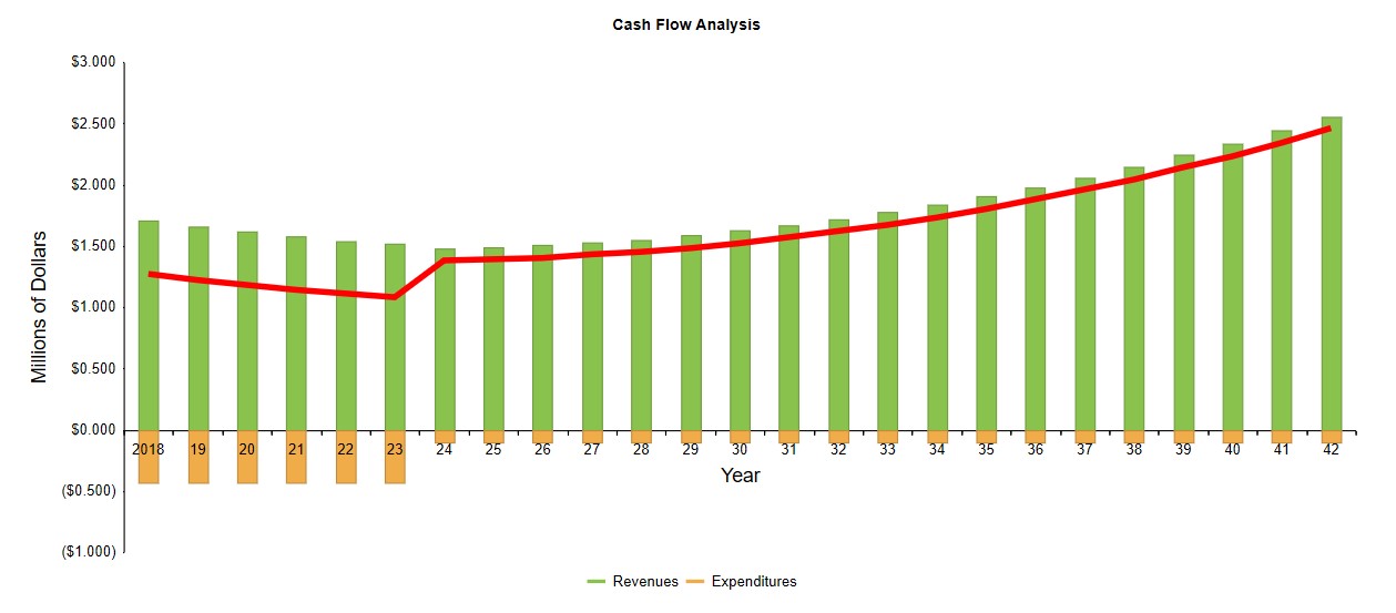
Clicking on a revenue bar shows the detailed breakout of impacts due to federal and state/local taxes,
broken out by households and businesses.
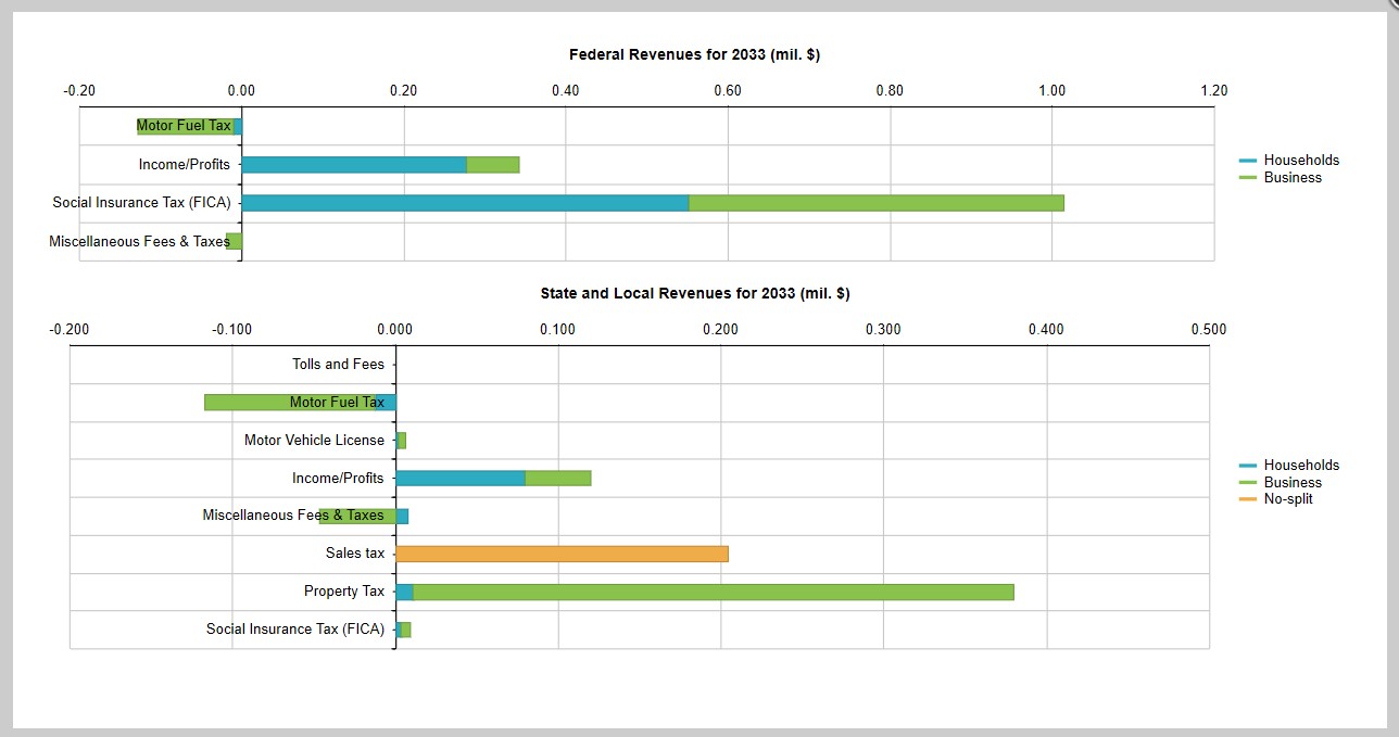
Likewise, clicking on a cost bar shows the detailed breakout of expenditure impacts for the project.
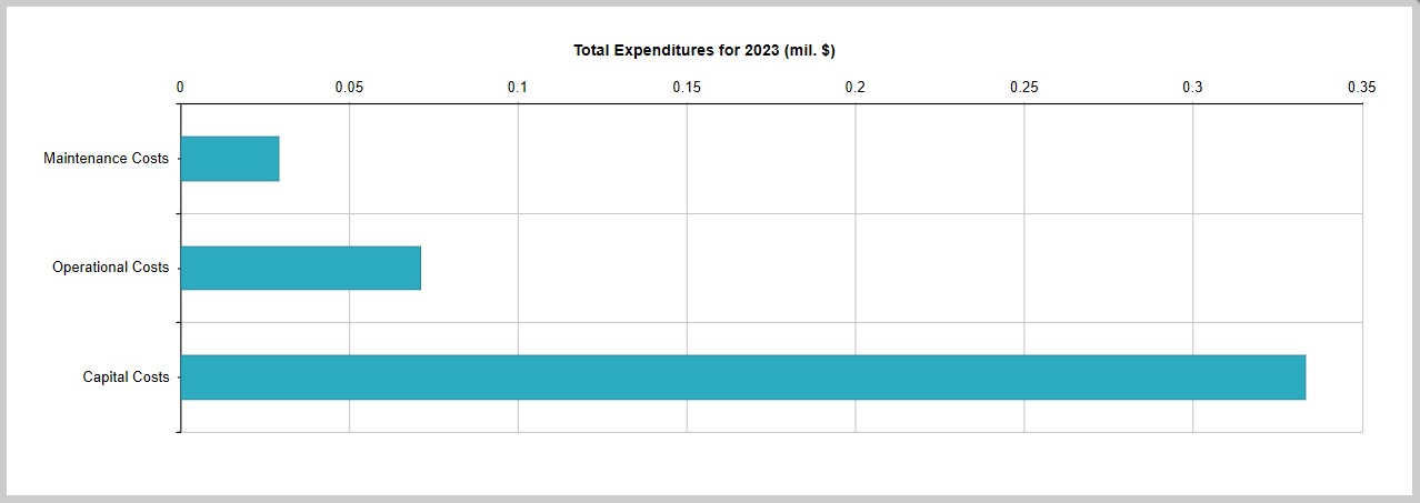
Revenues Tab
Under the Revenues tab, select a Region and Year to see projected revenues. Like other matrix tables, clicking
the plus or minus sign in the upper left will expand or collapse all rows, and clicking the Excel symbol in the upper
right will export the data shown as a spreadsheet that can be saved.
Impact Type |
The Impact type menu allows you to view the total impacts or filter the results to view only construction, operational, contingent development,
or market access impacts.
|
Cash Flow |
This control allow you to select with real or Nominal (Future $) for Cash Flow.
|
Inflation Rate |
This control allow you to change the inflation rate used in your analysis.
|
Note that Sales Tax is NA under the Household and Business disaggregate columns because the foundational IMPLAN data underlying TREDIS calculations does not provide the incidence split between the two entities.
Cost and Revenue Sharing
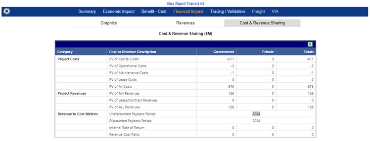
Undiscounted Payback Period and Discounted Payback Period show the year that cumulative revenues top cumulative
costs. Discounts here are the first discount rate specified on the Results settings page.
| TREDIS 6.0 User Manual | Return to Contents |
Results - Tracing/Validation
Introduction
TREDIS allows you to filter your results using the drop down menu controls at the top of many of the Tracing/Validation results screens. Note that not all controls appear on each results screen.
Economic Activity |
This control allows you to adjust the results view to look at the comparison between project versus base, the base results, or the
project results.
|
Periods |
This control allows you to filter your results for specific periods from your analysis as set on the Timing Screen.
|
Industry Aggregation |
The Industry Aggregation menu allows you to adjust the industry details viewed in the results:
|
Impact Type |
The Impact type menu allows you to view the total impacts or filter the results to view only construction, operational, contingent development, or market access impacts.
|
Graphics Tab
Summary of the travel changes in your project. Click on metric in the legend to toggle it on or off.
In the following descriptions, the cost savings in the variable described are reported, not the level itself. So, for example, the Crew Cost line item doesn’t describe the costs of the crew in the Base or Project alternative; the Crew Cost line item is the difference (Base minus Project) between the two alternatives.
Overview of Travel
Primary measures of performance, including miles per trip, minutes per trip, speed,
and fraction of miles traveled in congestion.
The dropdown controls at the top left include a Breakdown and a Perspective dropdown. The Breakdown options
include By Purpose and By Mode, while the Perspective options include Vehicle or Passenger/Ton Changes
in performance metrics between the base and project scenarios by year.
Change in Project Costs
Differences between project costs by facility type, year, and subcategory of cost.
Change in Travel Characteristics
Changes in performance metrics between the base and project scenarios by year.
Clicking on a year expands the table to show the changes in travel characteristics for each mode-purpose combination for that year. This report is helpful to verify that you have entered in your travel data correctly.
Positive numbers indicate savings in trips, mileage, or time saved. That is, the level of the Project alternative is less than the level of the Base alternative. Negative numbers in this report indicate dissavings of these, i.e., an increase in activity.
Cost Savings by Type
Cost savings by mode-purpose combination and type.
To see how the cost savings are allocated across each cost category, click on a specific year. In this expansion view, we see which cost elements are the primary sources of savings in the selected year.
- Passenger Cost (In Vehicle) ‐ Value of time of passengers for time spent in a vehicle.
- Passenger Cost (Out of Vehicle) ‐ Value of time of passengers for time spent outside the vehicle.
- Crew Cost ‐ Value of time for drivers or other vehicle crew.
- Freight Cost ‐ Cost of freight goods being transported. This field is deprecated and set to 0 for results run as of March 2021; for projects run previously, it will maintain the previous cost estimated until the project has results run again.
- Freight Cost (Reliability) ‐ Costs due to addressing unreliability in goods movements that are passed on to shippers and receivers of freight.
- Freight Cost (Delay) ‐ Costs due to delay in delivery of goods that is passed on to shippers and receivers of freight.
- Reliability Cost ‐ Value of time for passengers and crew spent buffering trips in order to arrive on time under unreliability circumstances.
- Fuel Cost w/Taxes ‐ Costs, including taxes, of fuel.
- Veh O&M Cost ‐ Operations and maintenance costs of vehicles, not including fuel.
- Fee per Vehicle Trip ‐ Charges and‐ fees incurred on a trip basis (e.g., road tolls, parking).
- Fee per Passenger Trip ‐ Charges and fees incurred on a passenger trip basis (e.g., transit or taxi fares).
- Fee per Passenger Mile ‐ Charges and fees incurred on a passenger mile basis (e.g., transit or taxi fares).
- Fee per Vehicle Mile ‐ Charges and fees incurred on a vehicle mile basis (e.g., mileage-based fees).
- Safety Cost ‐ Societal benefits (or disbenefits) from averted fatalities, injuries, and property damage.
- Environmental Cost ‐ Societal benefits (or disbenefits) from averted emissions, including GHGs.
Note that the Safety Cost reported here is a societal benefit, and not the same figure as the Safety impacts reported on the Project Impacts by Industry report. (Those are completely economic benefits and are calculated in a separate procedure.)
Transportation Services Accounting Summary
Accounting for revenues, costs, and driver income for TNC modes.
In the example below, TNC operations are expected to collect $200,000 more in the Project alternative than in the Base alternative.Of the $200,000, TNC management takes 25% of gross revenues, or $50,000 of revenues. Operating costs ($5,376) are then subtracted from the remainder, and finally Driver Income (via Driver Earnings from Fares) is what remains after operating costs. If the driver is operating at a personal loss for any reason, the improvement or worsening loss of this personal is shown in the line Driver Non-Fare Assets or Income, until the driver is no longer losing money by driving, after which it is reflected in income.
Results from this report inform the Costs Savings by Industry and Project Impacts by Industry reports. Total revenues to drivers and TNC companies are taken out of household or employer budgets.
- This report is only available if a TNC mode has been selected (on the Modes screen).
- The Company Share field (which determines share of revenues going to management company) is set in Modes screen > Adjust Mode Factors window > Other Costs tab.
- TNC charges can be entered as Per Passenger Mile charges or Per Passenger Trip charges in the Travel screen > Charges, Tolls, Fees tab.
Cost Savings by Industry
Savings (as shown in Costs Savings by Type) by industry and
special aggregate groups (e.g., household).
Positive numbers indicate savings in dollars or time valued in dollars. That is, the level of the Project alternative is less than the
level of the Base alternative. Negative numbers in this report indicate dissavings of these, i.e., an increase in money spent (or
time valued in dollars).
The bulk of the line items in this report show how savings go to specific industries, defined by NAICS code. You can control
the degree of industry detail in the Results screen control panel. (Available via the Gear symbol on the top left once reports have already been run.)
- If you choose the highest degree of detail (in the Results settings panel, certain sectors of
reporting will not correspond directly to a NAICS code.
- Non-industry sectors defined by IMPLAN have a description beginning Not an Industry….
- Government sectors defined by IMPLAN have a description Employment and payroll of….
- Household Value of Time Benefit is time savings, monetized.
- Societal & Environmental Benefits are monetized.
- Transit Operating Expenses are not used in the benefit-cost analysis or economic model because they are typically assumed to be entered as spending input on the Costs screen.
Project Impacts by Industry
Savings here serve as inputs into the economic
model and reflected, finally, in the Economic Impact reports (Results screen ‐ Economic Impact tab).
Positive numbers indicate savings in dollars or time valued in dollars. That is, the level of the Project alternative is less than the
level of the Base alternative. Negative numbers in this report indicate dissavings of these, i.e., an increase in money spent (or
time valued in dollars).
Impacts are summarized by columns describing their source. based on four categories of potential impact sources.
- Travel Cost Savings are produced by changes between Base and Project alternatives entered on the Travel page. These might include savings for households and industries through a variety of mechanisms including savings of time on business travel, fuel, and vehicle operating costs. These do not include economic impacts of averted crashes, fatalities, and injuries, which are tallied under the Safety column.
- Contingent Development impacts are produced directly by items entered on the Contingent Development tab of the Access page. These represent impacts that might accrue due to considerations outside of a travel model, such as the establishment of a new business venture due to improved travel.
- Additional Potential Output from Market Access comes from the Intercity Access tab of the Access page. These include productivity improvements stemming from enhanced employment opportunities, business-to-business opportunities, and port efficiency.
- Safety impacts are produced by improved economic outcomes from averted fatalities, injuries, and property damage, including reallocation of medical care costs back to payees (both firms and households), lost productivity due to injury, and insurance costs. Impacts listed here are for economic impact purposes and not for societal benefit calculations â€" those figures are shown in the Cost Savings by Type report.
- Driver Budget (Not Reallocated) represents the net to the drivers of TNCs. This is the same as the Driver Income line from the Transportation Services Accounting Summary.
- Household Budget (Reallocated) represents the net to the Household sector, with money reallocated to other sectors to where spending will occur in the economic model. These typically include vehicle operating costs and fuel costs for private travel (or half of commute travel).
- Household Budget (Not Reallocated) represents the net to the Household sector, with money not reallocated to other sectors in the economic model, typically because the money is collected by an agency.
- Transit Operating Expenses represents the net change of spending on operating transit. These figures are not used in the economic model because they are typically assumed to be entered (and impacts determined) by spending input on the Costs screen.
Market Access Impacts by Source
Impacts of the market access impacts, tracing the effects of inputs on the Access page, Intercity Access tab.The Access Characteristics Summary shows how the inputs are transformed into single metrics expected by the estimation functions and shows the difference between the Base and Project alternatives as a percentage.
To calculate the compound metrics, decay factors are used to weight the population or employment in each band — that is, the additional quantity present in a larger region relative to the next smaller input quantity. For example, if the population within 40 minutes is 1,000,000 and the population within 60 minutes is 1,200,000, the population in the 40-60 minutes band is 200,000.
Local Market (population) is a weighted average of the population bands given in the Access page to represent consumer and labor markets. The measure is:
100% of pop within 40 minutes + 40% of pop 40-60 minutes
Regional Same Day Market (employment) is a metric reflecting improved access to same-day freight deliveries and business relationships. The metric is a ratio where a weighted average of the employment bands is the numerator and the employment within one hour of the county center is the denominator:
(100% of 1- to 2-hr employment + 85% of 2- to 3-hr employment + 15% of 3- to 4-hr employment) / 0- to 1-hr employment
A separate ratio using the population inputs is used to calculate access to population that affects visitor services industries.
Gross Business Attraction from Market Access Improvement shows nominal dollar impacts, broken down by source of market access impact for the last year of operations modeled. These changes are split between productivity changes and business attraction (as higher local productivity leads to relocation of business from other locations).
Market Access Impacts by Industry
These represent direct economic impacts from Gross Business Attraction from Market Access Improvement (as described above in Market Access Impacts by Source), spread across all operations years and broken down by industry.
Impacts depend on the industry mix and scale for the County of Focus for each Region modeled, not for the entire Region.
Intercity Access impacts phase in over time as the local economy reacts to accessibility changes. This leads to much smaller impacts in early operation years.
| TREDIS 6.0 User Manual | Return to Contents |
Results - Equity
The Equity section provides insight regarding the extent of economic hardship (poverty, low income, high unemployment, lack of car ownership)
and historically underserved populations (elderly, physical disability, racial/ethnic minority status) among the study regions. This is expressed
in terms of both baseline context and project impact.
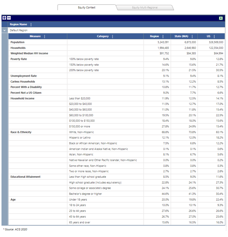
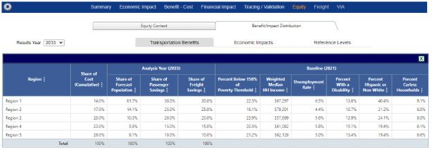
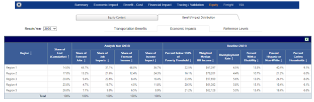
In this report, the distribution of regional economic impacts reported under Economic Impacts reports are presented alongside equity measures.
The Measures shown for the Modeled Regions take each Region defined in the model as an observation. The State and National geographies take each county in the state or the US as the unit of observation.
For each equity measure, three measures are shown:
However, within the State, Region 1 ranks somewhat better, since among all the states’ counties, 7.5% is the cutoff for the top 20th. Region 1’s 6.5% unemployment rate is below that and thus better than at least 20% of the counties in the state (assuming Region 1 doesn’t include any of those counties).
Nationally, however, Region 1 would still be higher than 80% of counties, which we can say because the top 20th percentile is only 5.9% for all counties in the US for the data from year 2021 in this example.
Equity Context
The Equity Context tab shows current baseline conditions for each study region. This includes rates of economic hardship among each region’s
population (poverty, low income, high unemployment, lack of car ownership) and the percentage shares of historically underserved populations
(elderly, physical disability, racial/ethnic minority, non-citizen) living in each region. These measures are compared to state and national figures,
so you can see how each region compares to wider area averages. This provides baseline insight for interpreting the impact findings presented
in the next tab.
Equity – Benefit/Impact Distribution
In addition to simply comparing a project’s regions directly in terms of their populations, the Benefit/Impact Distribution
reports show how the benefits and impacts of a project are distributed to the regions, along with some equity measures
of interest. In this way, you may quickly see whether the regions that enjoy benefits or impacts are the same regions
that may have the greatest need.
Transportation Benefits
In this report, the distribution of regional benefits reported under Benefit – Cost reports are presented alongside equity measures.
The Results Year drop-down can be used to see specific operations years.
The Results Year drop-down can be used to see specific operations years.
Share of Cost (Cumulative) – Percentage of all costs as entered in the Cost page, summed across all Construction Years
Share of Forecast Population – Percentage of the forecasted population (in the Base alternative) for the Analysis Year
Share of Passenger Savings – Percentage of total savings experienced by modes with a purpose of Business, Personal, or Commute
Share of Freight Savings – Percentage of total savings experienced by modes with Freight purpose
The columns under the Baseline rubric reiterate the equity measures for each region for convenient comparison with shares of savings.
Share of Forecast Population – Percentage of the forecasted population (in the Base alternative) for the Analysis Year
Share of Passenger Savings – Percentage of total savings experienced by modes with a purpose of Business, Personal, or Commute
Share of Freight Savings – Percentage of total savings experienced by modes with Freight purpose
The columns under the Baseline rubric reiterate the equity measures for each region for convenient comparison with shares of savings.
Economic Impacts
In this report, the distribution of regional economic impacts reported under Economic Impacts reports are presented alongside equity measures.
The Results Year drop-down can be used to see specific operations years.
Share of Cost (Cumulative) – Percentage of all costs as entered in the Cost page, summed across all Construction Years
Share of Forecast Jobs – Percentage of the jobs (in the Base alternative) for the Analysis Year
Share of Job Impacts – Percentage of the change in total jobs that are an impact of the Project alternative in the Analysis Year
Share of Forecast Income – Percentage of the labor income (in the Base alternative) for the Analysis Year
Share of Income Impact – Percentage of the change in total labor income that is an impact of the Project alternative in the Analysis Year
The columns under the Baseline rubric reiterate the equity measures for each region for convenient comparison with shares of savings.
Share of Cost (Cumulative) – Percentage of all costs as entered in the Cost page, summed across all Construction Years
Share of Forecast Jobs – Percentage of the jobs (in the Base alternative) for the Analysis Year
Share of Job Impacts – Percentage of the change in total jobs that are an impact of the Project alternative in the Analysis Year
Share of Forecast Income – Percentage of the labor income (in the Base alternative) for the Analysis Year
Share of Income Impact – Percentage of the change in total labor income that is an impact of the Project alternative in the Analysis Year
The columns under the Baseline rubric reiterate the equity measures for each region for convenient comparison with shares of savings.
Reference Levels
This report gives context to the Transportation Benefits and Economic Impact reports by showing the distribution for each of the equity variables of interest among the geographic units analyzed.The Measures shown for the Modeled Regions take each Region defined in the model as an observation. The State and National geographies take each county in the state or the US as the unit of observation.
For each equity measure, three measures are shown:
Top 20th – The cutoff point above which 20% of regions or counties have higher levels of the observed statistic
Median – The median observation for the statistic
Bottom 20th – The cutoff point below which 20% of regions or counties have lower levels of the observed statistic
Using the screenshots as an example, in any of the other Equity reports, you can see that Region 1 has an unemployment
rate of 6.5%. From the points shown in the Reference Levels for top 20th, median, and bottom 20th – 5.8%, 5.6%, and 5.0%,
respectively – you can see that 6.5% is relatively high among the regions modeled for this project.
Median – The median observation for the statistic
Bottom 20th – The cutoff point below which 20% of regions or counties have lower levels of the observed statistic
However, within the State, Region 1 ranks somewhat better, since among all the states’ counties, 7.5% is the cutoff for the top 20th. Region 1’s 6.5% unemployment rate is below that and thus better than at least 20% of the counties in the state (assuming Region 1 doesn’t include any of those counties).
Nationally, however, Region 1 would still be higher than 80% of counties, which we can say because the top 20th percentile is only 5.9% for all counties in the US for the data from year 2021 in this example.
| TREDIS 6.0 User Manual | Return to Contents |
Results - Freight - Transearch
Use the sub tabs at the top of the screen to detailed table views:
Freight Summary
This screen shows the composition of freight flows in both tons or dollars for the selected region in both graphical and tabular format by years. You can see inbound, outbound, internal and through flows of commodities in addition to the totals of all origin-destination options.
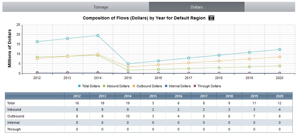
Flow by Mode
The Flow by Mode screen presents by mode, the tons of goods, dollar value of those goods, or the number of vehicles used to transport those goods, by year and also flow type (inbound, outbound, etc.)
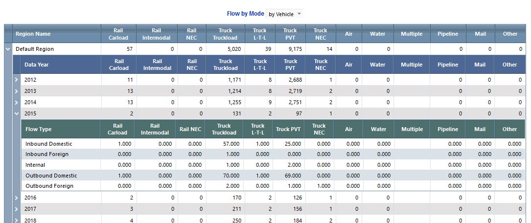
Mode-Commodity Mix
The Mode-Commodity Mix screen presents by mode, the tons of goods, dollar value of those goods, or the number of vehicles used to transport those goods, by year along with the detail commodities transported.
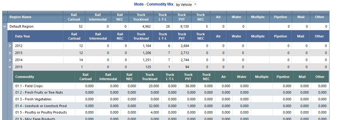
Trip Lengths
The Trip Lengths report breaks down the distances the commodities move, again as tons of goods, value of goods, or number of vehicles moving the goods, showing the breakdown in distance ranges, average, and estimated VMT.
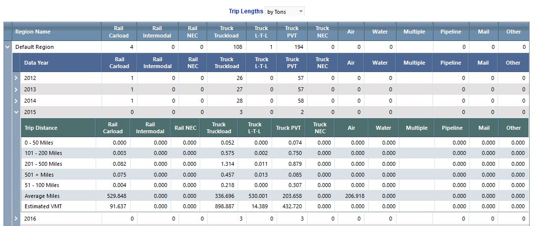
Top locations
The Top Locations chart, presents as either a bubble chart or a direction chart the relative flow of goods (as tons, value, or number vehicles) with the largest/darkest bubbles delineating the largest values and conversely the smallest/lightest bubbles representing the smallest values. The quantities to be presented are selected with the drop down menus for
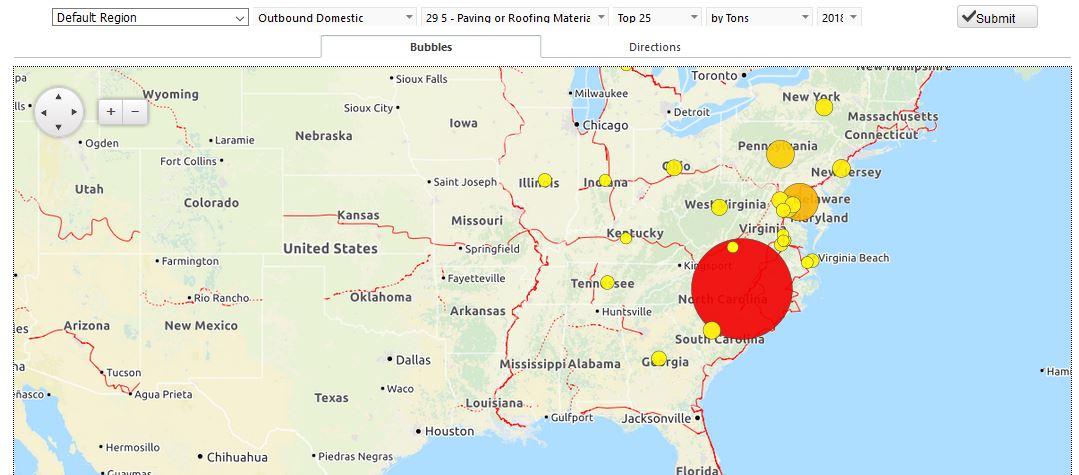
Economy Relationships
The Economy Relationships chart shows the trend for the top 7 commodities transported by value.
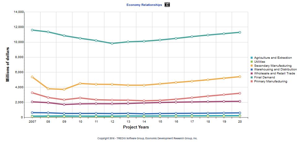
Freight Dependency
The Freight Dependency tab present the economic impacts (output, value added, income, and jobs) by industry for the region, direction, modes, commodities, and year selected, with the option to include labor match.
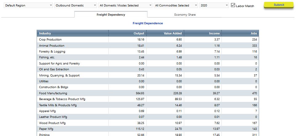
This screen shows the composition of freight flows in both tons or dollars for the selected region in both graphical and tabular format by years. You can see inbound, outbound, internal and through flows of commodities in addition to the totals of all origin-destination options.
Flow by Mode
The Flow by Mode screen presents by mode, the tons of goods, dollar value of those goods, or the number of vehicles used to transport those goods, by year and also flow type (inbound, outbound, etc.)
Mode-Commodity Mix
The Mode-Commodity Mix screen presents by mode, the tons of goods, dollar value of those goods, or the number of vehicles used to transport those goods, by year along with the detail commodities transported.
Trip Lengths
The Trip Lengths report breaks down the distances the commodities move, again as tons of goods, value of goods, or number of vehicles moving the goods, showing the breakdown in distance ranges, average, and estimated VMT.
Top locations
The Top Locations chart, presents as either a bubble chart or a direction chart the relative flow of goods (as tons, value, or number vehicles) with the largest/darkest bubbles delineating the largest values and conversely the smallest/lightest bubbles representing the smallest values. The quantities to be presented are selected with the drop down menus for
- Region
- Direction (inbound/outbound, total/domestic/international)
- Commodity of interest (or all commodities)
- Number of data points to show (top 5, 10, 25 (default), 50, 75, or 100)
- Value shown (tons, value, vehicles)
- and Year of interest
Economy Relationships
The Economy Relationships chart shows the trend for the top 7 commodities transported by value.
Freight Dependency
The Freight Dependency tab present the economic impacts (output, value added, income, and jobs) by industry for the region, direction, modes, commodities, and year selected, with the option to include labor match.
| TREDIS 6.0 User Manual | Return to Contents |
Results - Freight
Once the Freight Analysis has finished running, you will be left at the Summary Results screen. Press the Freight tab to view your freight results.
Freight Summary
This screen presents a summary of the total commodity flows by tons or value, depending upon which subtab is selected. Only the years selected on the settings page show values, so if more details are needed, you will need to rerun the freight analysis from the settings screen.
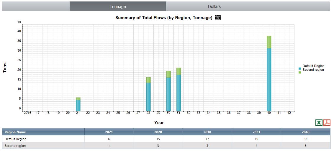
Clicking on a bar in the graph will bring up a popup window with a line graph showing the composition of freight flows in either tons or value as selected using the tab. Flows are shown as total, inbound (coming into the study region), outbound (exported from the region), internal (origin and destination within the study region), and through (origin and destination are external to the study region). This data is provided in both graphical and tabular formats both allowing for the export of the data.
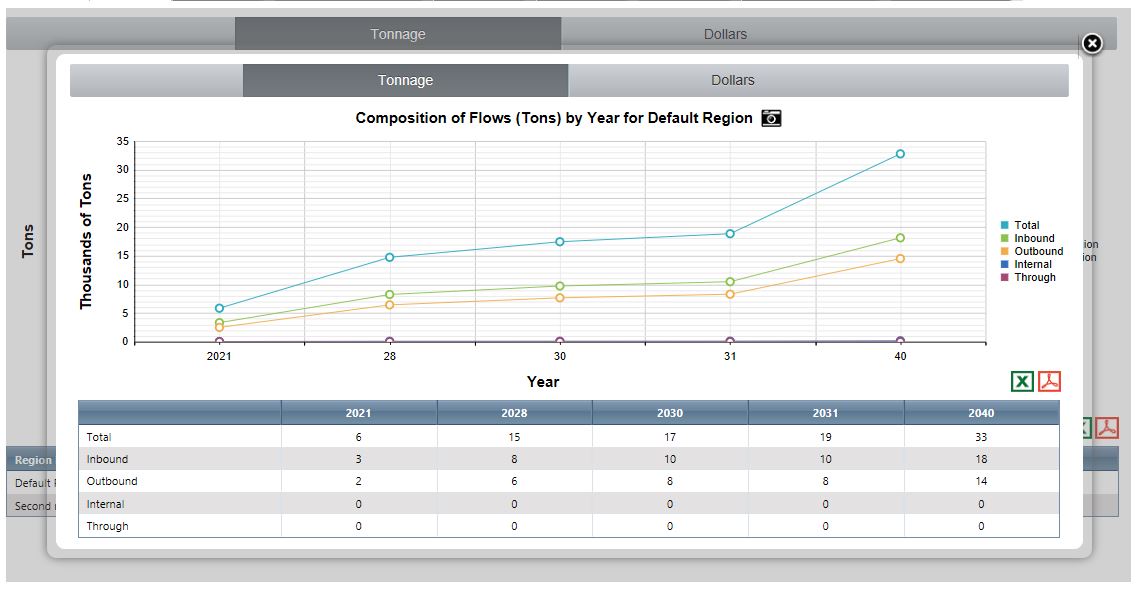
In a similar manner, if you hover over a data point on a line, you will see the value at that point. Clicking on the data point brings up another popup with the commodity details in both tabular and graphical formats:
Flow by Mode
The Flow by Mode screen presents by mode, the tons of goods, dollar value of those goods, or the number of vehicles used to transport those goods, by year and also flow type (inbound, outbound, etc.)
Mode-Commodity Mix
The Mode-Commodity Mix screen presents by mode, the tons of goods, dollar value of those goods, or the number of vehicles used to transport those goods, by year along with the detail commodities transported.
Trip Lengths
The Trip Lengths report breaks down the distances the commodities move, again as tons of goods, value of goods, or number of vehicles moving the goods, showing the breakdown in distance ranges, average, and estimated VMT.
Top locations
The Top Locations chart presents as either a bubble chart or a direction chart the relative flow of goods (as tons, value, or number vehicles) with the largest/darkest bubbles delineating the largest values and conversely the smallest/lightest bubbles representing the smallest values. The quantities to be presented are selected with the drop down menus for
All locations
The All Locations tab provides baseline vFreight data for your study region, based on the settings you select in this tab for commodity flow direction (inbound/outbound domestic/international), commodities to view, domestic mode type, foreign mode type (for international flows), and foreign trade partner. Pressing the submit button processes this baseline data and is presented as a set of tables and maps (for more detailed user instructions please click here):
Economy Relationships
The Economy Relationships chart shows the trend for the top 7 commodities transported by value.
Freight Dependency
The Freight Dependency tab present the economic impacts (output, value added, income, and jobs) by industry for the region, direction, modes, commodities, and year selected, with the option to include labor match.
This screen presents a summary of the total commodity flows by tons or value, depending upon which subtab is selected. Only the years selected on the settings page show values, so if more details are needed, you will need to rerun the freight analysis from the settings screen.
Clicking on a bar in the graph will bring up a popup window with a line graph showing the composition of freight flows in either tons or value as selected using the tab. Flows are shown as total, inbound (coming into the study region), outbound (exported from the region), internal (origin and destination within the study region), and through (origin and destination are external to the study region). This data is provided in both graphical and tabular formats both allowing for the export of the data.
In a similar manner, if you hover over a data point on a line, you will see the value at that point. Clicking on the data point brings up another popup with the commodity details in both tabular and graphical formats:
Flow by Mode
The Flow by Mode screen presents by mode, the tons of goods, dollar value of those goods, or the number of vehicles used to transport those goods, by year and also flow type (inbound, outbound, etc.)
Mode-Commodity Mix
The Mode-Commodity Mix screen presents by mode, the tons of goods, dollar value of those goods, or the number of vehicles used to transport those goods, by year along with the detail commodities transported.
Trip Lengths
The Trip Lengths report breaks down the distances the commodities move, again as tons of goods, value of goods, or number of vehicles moving the goods, showing the breakdown in distance ranges, average, and estimated VMT.
Top locations
The Top Locations chart presents as either a bubble chart or a direction chart the relative flow of goods (as tons, value, or number vehicles) with the largest/darkest bubbles delineating the largest values and conversely the smallest/lightest bubbles representing the smallest values. The quantities to be presented are selected with the drop down menus for
- Region
- Direction (inbound/outbound, total/domestic/international)
- Commodity of interest (or all commodities)
- Number of data points to show (top 5, 10, 25 (default), 50, 75, or 100)
- Value shown (tons, value, vehicles)
- and Year of interest
All locations
The All Locations tab provides baseline vFreight data for your study region, based on the settings you select in this tab for commodity flow direction (inbound/outbound domestic/international), commodities to view, domestic mode type, foreign mode type (for international flows), and foreign trade partner. Pressing the submit button processes this baseline data and is presented as a set of tables and maps (for more detailed user instructions please click here):
Economy Relationships
The Economy Relationships chart shows the trend for the top 7 commodities transported by value.
Freight Dependency
The Freight Dependency tab present the economic impacts (output, value added, income, and jobs) by industry for the region, direction, modes, commodities, and year selected, with the option to include labor match.
| TREDIS 6.0 User Manual | Return to Contents |
Results - VIA
Coming Soon
| TREDIS 6.0 User Manual | Return to Contents |
Glossary
| Term | Definition | ||||||||||||||||
| Alternative | Within a TREDIS project, alternatives such as Base (no-build) and Project (build) are compared | ||||||||||||||||
| Analysis Type | TREDIS adapts the user inputs and available results to match where in the transportation planning cycle the user project falls. In addition to the Advanced Mode, TREDIS includes Public Policy, Vision Planning, Prioritization, Alternatives Analysis, Single Project, Existing Facility, and Asset Management Types. | ||||||||||||||||
| Access | See Market Access | ||||||||||||||||
| BCA | Benefit Cost Analysis. Click here for detailed explanation | ||||||||||||||||
| Buffer Time | Refers to the hours that travelers must set aside for each vehicle trip in addition to their travel time in order to arrive on-time 95% of trips. Average buffer time per trip is related to average travel time per trip by the buffer time index. TREDIS can estimate needed buffer time per trip based on the information you provide on total Trips, total VHT, and percent of VMT congested (V/C > .9). | ||||||||||||||||
| Constant Dollar Year | The adjusted value of currency used to compare dollar values from one period to another. | ||||||||||||||||
| Construction Period | The schedule years when a project's construction activities occur. This period ranges from the Construction Start Year to the Construction End Year | ||||||||||||||||
| Contingent Development | Refers to discrete jobs or business sales attracted to the region due to the transportation improvement – the development of this economic activity is contingent on completion of the project. Contingent development within the market access inputs section of TREDIS can be used when the agency has more specific information on land development or job attraction that should be included as well as estimates from transportation cost savings and expansions of the labor market or same day deliver market areas. | ||||||||||||||||
| Contract | TREDIS organizes subscriptions using the concept of contracts. The contract contains information about the geographies the user may access and time period the subscription is active. | ||||||||||||||||
| Costs | Costs are the project expenditures made during the Construction Period and then the operating and maintenance expenditures during the Operations Period. | ||||||||||||||||
| Cost Elements: |
|
||||||||||||||||
| CO2 | Carbon Dioxide (pollutants) | ||||||||||||||||
| Custom Mode | A custom mode is a user created mode, based on an existing mode which can have different default values. Custom modes are shared among all members of the user's account, with the user who created the custom mode uniquely able to edit the default values. | ||||||||||||||||
| Direct Impact | The effect of cost savings to system users under the transportation scenario modeled, or spending by the operator or constructing entity of a project or service. | ||||||||||||||||
| Discount Rate | Cost of capital (interest rates). Note: TREDIS uses the default values of 3% and 7%, which corresponds to the values typically used in grant applications, although the user may change these values prior to running the analysis on the Results - Settings screen. | ||||||||||||||||
| EIA | Economic Impact Analysis. Click here for detailed explanation | ||||||||||||||||
| Environmental Factors | This deals with emissions generated by the vehicles in the project. Factors include tons of emissions (VOC, SO2, NOX, PM, and CO2) per vehicle mile traveled both free flow and congested, along with the cost per ton of these pollutants. | ||||||||||||||||
| FIA | Financial Impact Analysis. Click here for detailed explanation | ||||||||||||||||
| Fraction Congested | Fraction of time all vehicles for a specific mode-purpose are experiencing congestion (values range from 0 - 1.0) | ||||||||||||||||
| Fraction of Trips: Incoming | Fraction of trips (0 - 1.0) that originate outside the study region and end in the study region | ||||||||||||||||
| Fraction of Trips: Internal | Fraction of trips (0 - 1.0) that originate in the study region and also end in the study region | ||||||||||||||||
| Fraction of Trips: Outgoing | Fraction of trips (0 - 1.0) that originate inside the study region and end outside the study region | ||||||||||||||||
| Fraction of Trips: Through | Fraction of trips (0 - 1.0) that originate outside the study region and end outside the study region | ||||||||||||||||
| Indirect Impacts | The effect of spending by the suppliers to business users benefiting from system improvements, or suppliers of operators or constructing entities of a project or service. | ||||||||||||||||
| Induced Impacts | The effect of household spending due to additional employment and payroll generated by direct and indirect impacts. | ||||||||||||||||
| Labor Income | Labor Income includes employee compensation and proprietor income. In TREDIS, it represents the additional wages, salaries, and benefits for employees and new income for proprietors from the scenario analyzed. | ||||||||||||||||
| Labor Market | The labor market affected by a project is considered to be the number of residents within a 40 minute trip of an employment center affected by the project. TREDIS default labor market values are based on the population within a 40 minute drive-time from the population-weighted centroid of a county. On the Summary graphic, TREDIS shows the percent improvement which you indicated your project is expected to provide. | ||||||||||||||||
| Linked Area | Regions directly connected to study region, defaults to geographies within study region, but may be overwritten. (Contact your account manager to add linked areas that are outside your subscribed account regions) | ||||||||||||||||
| Local Market | Approximate 40-minute commute time (way). The threshold at which most employees are willing to travel. | ||||||||||||||||
| Market Access | Translates changes in market access and intermodal connectivity into effects on agglomeration, dispersion and scale economies for industry sectors. It applies calculation methods backed by peer-reviewed publications for estimating wider economic impacts. | ||||||||||||||||
| Mode | Transportation type, such as passenger car, truck, and bus used in the Project analysis | ||||||||||||||||
| NOX | Nitric Oxide and Nitrogen Dioxide (pollutants) | ||||||||||||||||
| Occupational Aggregation | Refers to the number of digits of Standard Occupational Classification (SOC) codes to use when reporting economic impacts by occupation. The SOC system is developed and published by the U.S. Bureau of Labor Statistics and used for their reporting. TREDIS offers 2-, 3-, and 4-digit SOC Code aggregation. | ||||||||||||||||
| O & M | Operations and Maintenance - see Cost Elements for Ongoing Operations, and Maintenance and Rehabilitation. | ||||||||||||||||
| Operations Period | The period of time when the transportation system is in operation and is incurring operating and maintenance costs. This period ranges from the Operations Start Year to the Operations End Year. | ||||||||||||||||
| Output | Output represents the value of industry production. For manufacturers, this would be sales plus/minus change in inventory. For service sectors production, output is simply the value of sales. For Retail and wholesale trade, output is represented by gross margin and not gross sales. Margin is sales receipts less the cost of goods sold. | ||||||||||||||||
| Period | A time period specified at the Project Level, defined solely by its travel demand characteristics. Multiple periods may be used to model differences in peak vs. off-peak or seasonal differences resulting from road closures. | ||||||||||||||||
| Period Veh-Trips | The number of one way trips made by all vehicles during the period (annually for example) | ||||||||||||||||
| PM | Particulate matter (pollutants) - complex mixture of extremely small particles and liquid droplets in air. Particle pollution is made up of a number of components, including acids (such as nitrates and sulfates), organic chemicals, metals, and soil or dust particles. | ||||||||||||||||
| Productivity | The average measure of the efficiency of production, which is expressed as the ratio of the outputs to the inputs as used in the production process, i.e. output per unit of input. | ||||||||||||||||
| Project | The major unit of a TREDIS analysis defined by certain parameters being held constant. It has the following features: (1) the geography (Region) is constant over the entire analysis, (2) all Alternatives within the Project have the same time horizon (that is, the same Construction Period and Operations Period), and (3) certain parameters such as the discount rate, are "fixed" across Alternatives when they are being compared. | ||||||||||||||||
| Project Group | TREDIS allows the user to organize collections of projects in groups. The criteria for organizing is up to the user and may be elements such as user projects, team projects, archived projects (for saving older projects), etc. | ||||||||||||||||
| Purpose | Trip purposes are used to classify why a trip is taken and is associated with a mode to form a mode-purpose combination. The trip purposes will fall into one of the following five categories: Business, Personal, Commute, Freight, or No Split (which is the combination of the previous four selections.) | ||||||||||||||||
| Results Year | Year used for presenting TREDIS results, typically in the future | ||||||||||||||||
| Same-Day Market | Approximate 180-minute (3-hour) drive time for a same day truck delivery of goods. Allows for delivery and truck return to warehouse the same day. | ||||||||||||||||
| STCC | The Standard Transportation Commodity Code (STCC) is a publication containing specific product information used on waybills and other shipping documents. A STCC code is a seven digit numeric code representing 38 commodity groupings. | ||||||||||||||||
| SO2 | Sulfur Oxides (pollutants) | ||||||||||||||||
| Study Region | Geographic areas where the Build Alternative takes place. These study areas may be as small as a zip-code or as large as a collection of states. A project may have 1 or more Regions (up to 10). | ||||||||||||||||
| Supply Chain | Refers to the same day delivery market for an employment center modeled by the project. It conversely considers the establishments that can serve your employment center with same day delivers. TREDIS estimates Supply Chains based on the employment at establishments within a 3 hour drive time. Default values for supply chain area employment are based on the employment-weighted centroid of a county. On the Summary graphic, TREDIS shows the percent improvement which you indicated your project is expected to provide. | ||||||||||||||||
| Terminal | An intramodal transfer facility such as an airport, marine port, or rail facilities (passenger and freight) | ||||||||||||||||
| Time/Value Factors | Default values used by TREDIS to address costs per crew member, passenger, and freight logistics, as well as buffer time costs and out of vehicle transfer costs | ||||||||||||||||
| Travel Characteristics | Translates changes in traffic volumes, vehicle occupancy, speed, distance, reliability and safety into direct cost savings for household and business travel. It applies practices for travel modeling and economic valuation that are widely accepted by metropolitan, state and federal agencies. | ||||||||||||||||
| TREDIS | Transportation Economic Development Impact System | ||||||||||||||||
| Truck L-T-L | Truck L-T-L refers to Less than Truckload shipping. This Mode is used to describe trucks used where a shipment does not require a full 48- or 53-foot trailer. Examples are lift gate and residential pickups and deliveries, etc. | ||||||||||||||||
| Truck PVT | Refers to "Private" truck freight. | ||||||||||||||||
| Truck NEC | Refers to truck freight "Not Elsewhere Classified." | ||||||||||||||||
| Useful Life | The useful life of a facility describes the number of years after which a facility is considered to be obsolete and in need of replacement. TREDIS uses information on the useful life of project investment categories to determine the residual value of those investments at the end of the analysis period. At the completion of construction, investments begin depreciating at a rate tied to the useful life factor. | ||||||||||||||||
| Value Added | Value Added changes from a project can also be considered as changes in Gross Regional Product or GDP. Value Added is the difference between an industry’s or establishment’s total output and the cost of intermediate inputs. It consist of employee compensation, taxes on production and imports less subsidies, and gross operating surplus (similar to profit). | ||||||||||||||||
| VHT | Vehicles Hours Travelled | ||||||||||||||||
| VMT | Vehicle Miles Travelled | ||||||||||||||||
| VOC | Volatile Organic Compounds (pollutants) |
| TREDIS 6.0 User Manual | Return to Contents |
 TREDIS Software Group EBP US, Inc. 155 Federal Street, Suite 600, Boston, MA 02109 Telephone 617.303-0424 info@tredis.com www.tredis.com |
 |